1  Perbandingan Kategori

Perbandingan antar kategori dalam data dapat divisualisasikan dengan berbagai jenis chart untuk mempermudah analisis dan interpretasi. Bar Chart adalah metode paling umum, sementara variasi seperti Stacked Bar, Paired Bar, dan Diverging Bar menawarkan pendekatan berbeda tergantung pada kebutuhan. Bab ini membahas berbagai chart untuk perbandingan kategori, beserta kondisi data yang sesuai, tujuan visualisasi, serta kelebihan dan kekurangannya.

Data

• Placement Prediction Dataset

• Mobile Apps ScreenTime Analysis

• Electric Vehicle Population

• S&P 500, ETF, FX & Crypto (Daily updated)

• Discover Perspectives: HR Analytics Employee

data_ev <- read.csv("Data/EV_Population.csv")
data_survey <- read.csv("Data/employee-survey.csv", sep="|")

Ringkasan Chart

Jenis Chart	Kondisi Data	Tujuan Visualisasi	Kelebihan	Kekurangan
Bar Chart	Kategori	Perbandingan antar kategori	Mudah dipahami, fleksibel	Kurang efektif untuk banyak kategori
Lollipop Chart	Kategori	Variasi dari bar chart, lebih ringan	Visual lebih bersih, menyoroti perbedaan kecil	Kurang dikenal, kurang informatif untuk data kompleks
Paired Bar	Kategori	Membandingkan dua set kategori terkait	Memudahkan perbandingan langsung	Sulit dibaca jika terlalu banyak kategori
Stacked Bar	Kategori + Numerik	Menampilkan komposisi dalam kategori	Menghemat ruang, menampilkan distribusi	Sulit membandingkan sub-kategori
Diverging Bar	Kategori + Numerik	Distribusi dengan skala positif-negatif	Menampilkan keseimbangan atau perbedaan ekstrem	Sulit diinterpretasi jika terlalu banyak kategori
Dot Plot	Kategori + Numerik	Distribusi atau perbandingan	Lebih ringkas dari bar chart, menyoroti perbedaan kecil	Kurang umum digunakan
Marimekko/Mosaic	Dua Kategori	Proporsi dua variabel kategori	Efektif untuk melihat hubungan antar kategori	Sulit dibuat dan diinterpretasi
Unit Chart	Kategori + Proporsi	Menampilkan proporsi dengan ikon	Menarik secara visual	Kurang akurat untuk proporsi kecil
Waffle Chart	Kategori + Proporsi	Menampilkan proporsi dalam bentuk grid	Lebih estetis dari pie chart	Kurang akurat untuk nilai kecil
Heatmap	Matriks (Kategori + Numerik)	Representasi warna dari nilai numerik	Sangat efektif untuk data besar	Sulit untuk interpretasi nilai absolut
Gauge/Bullet	Numerik	Menampilkan indikator atau target	Bagus untuk KPI atau performa	Kurang efektif untuk perbandingan
Bubble Chart	Kategori + Numerik	Menampilkan hierarki atau hubungan	Mampu menunjukkan lebih dari dua dimensi	Sulit dibaca jika ada banyak data
Sankey Diagram	Kategori + Hubungan	Menampilkan aliran data antar kategori	Sangat efektif untuk alur proses	Sulit dibuat dan diinterpretasi
Waterfall Chart	Numerik	Menampilkan perubahan kumulatif	Bagus untuk analisis finansial	Tidak cocok untuk banyak kategori

1.1 Bar Charts

Bar chart (diagram batang) adalah salah satu teknik visualisasi data yang digunakan untuk membandingkan jumlah kategori berdasarkan ukuran tertentu. Dalam konteks ini, kita membandingkan jumlah kendaraan listrik dari berbagai brand.

Advanced

# Sort
data_ev_sorted <- data_ev %>%
  count(Make, name = "count") %>%
  arrange(desc(count)) %>%
  mutate(Make = str_to_title(Make))

# Top 3
top3 <- head(data_ev_sorted$Make, 3)

# Viz
chart <- 
  ggplot(data_ev_sorted, 
         aes(x = reorder(Make, count), y = count, 
             fill = ifelse(Make %in% top3, "steelblue", "gray50"))) +
  # Bar chart
  geom_bar(stat = "identity", width = 0.8) + 
  scale_fill_identity() +  # Apply warna tanpa legend
  
  # Label ujung bar
  geom_text(aes(label = count), hjust = -0.2, size = 2.5) +
  
  # Settings
  geom_hline(yintercept = -0.3, color = "black", linewidth = 0.5) +  
  coord_flip() +
  theme_minimal() +
  
  labs(title = "Dominasi Tesla dalam Pasar Kendaraan Listrik",
       subtitle = "Frekuensi Pendaftaran Kendaraan Listrik dari Berbagai Brand",
       x = "", 
       y = "") +
  theme(axis.text.y = element_text(size = 8, hjust = 1, face = "bold", 
                                   margin = margin(r = -25)),
        plot.title = element_text(hjust = -0.17, size = 14, face = "bold"),
        plot.subtitle = element_text(hjust = -0.13, size = 8),
        panel.grid.major.y = element_blank(),
        panel.grid.major.x = element_line(linetype = "dashed"),
        panel.grid.minor.x = element_line(linetype = "dashed")
  )

chart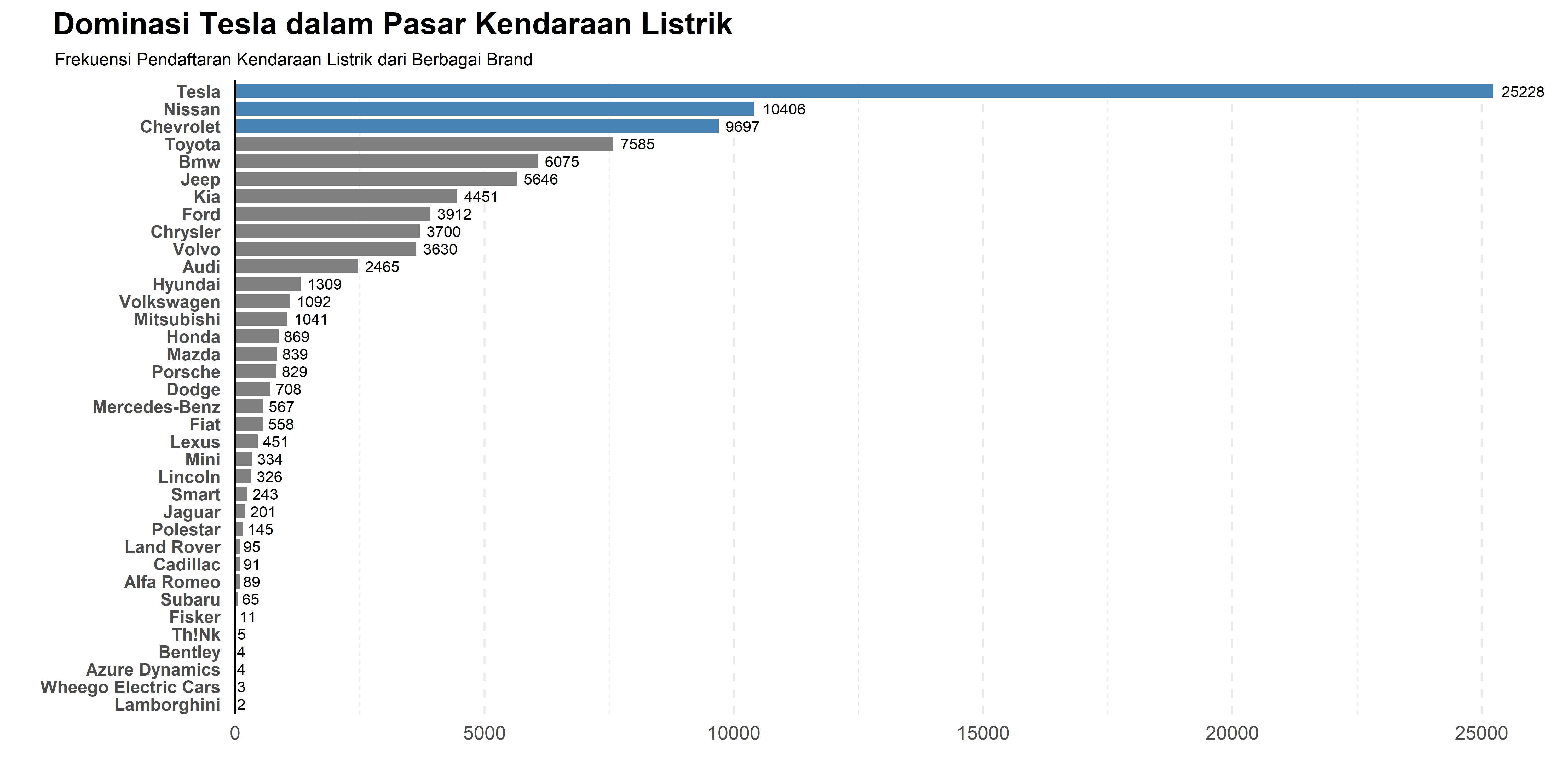

# Save Chart
ggsave("Chart/01_Bar.png", chart, dpi = 300, height = 5, width = 10)

Bar chart dalam ggplot2 bisa dikustomisasi untuk menyoroti informasi tertentu, seperti menampilkan top 3 brand, menambahkan frekuensi di ujung batang, atau mengubah warna kategori tertentu. Misalnya, dalam visualisasi ini, Tesla didominasi dengan warna biru, sedangkan brand lain berwarna abu-abu.

Sederhana

Namun, dalam bentuk sederhananya, bar chart cukup dibuat dengan menambahkan geom_bar().

ggplot(data_ev, aes(x = Make)) +
  # Bar chart
  geom_bar(fill = "#f1bb68")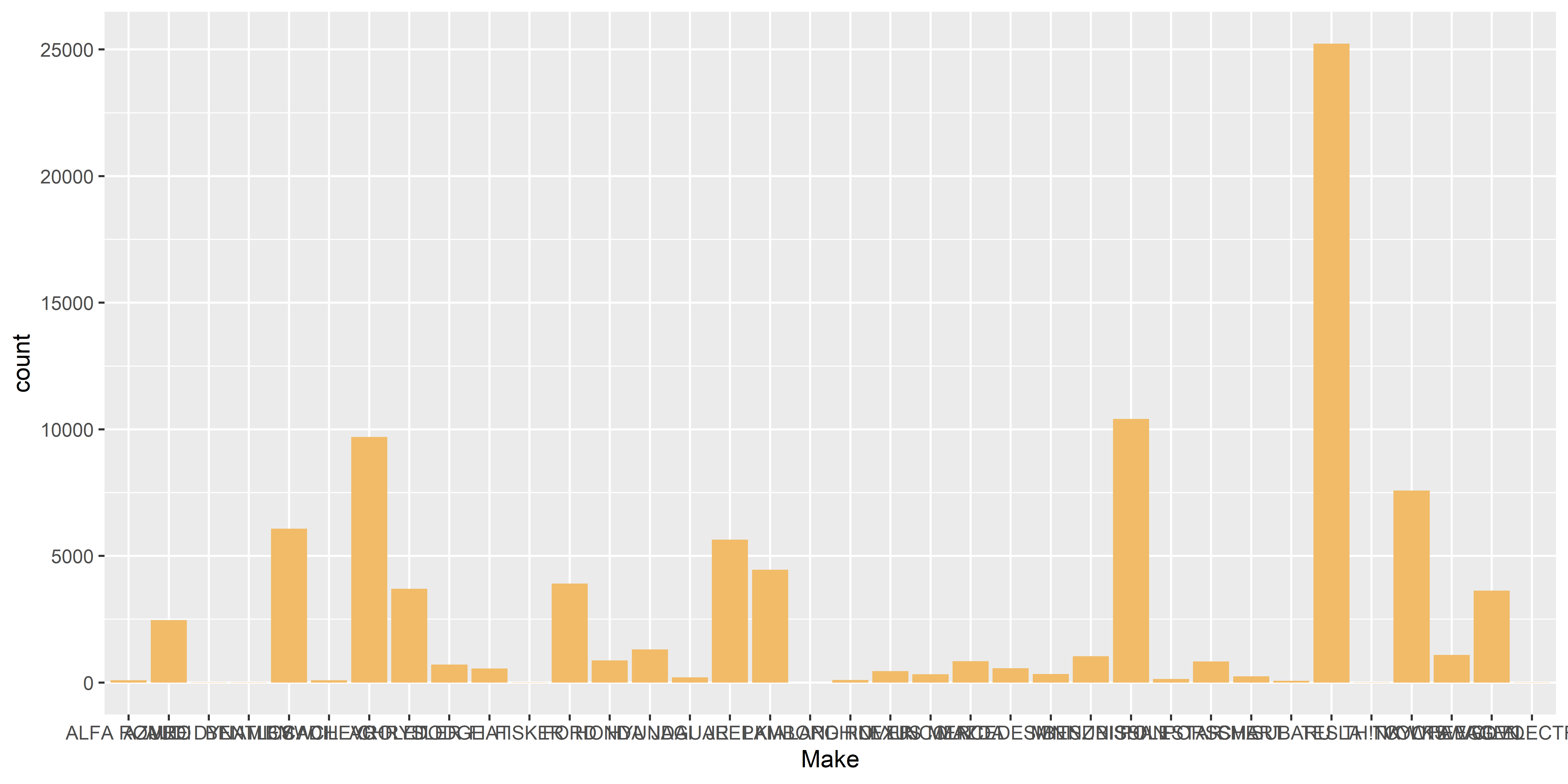

Untuk membuatnya horizontal, cukup menambahkan coord_flip().

ggplot(data_ev_sorted, 
       aes(x = reorder(Make, count), y = count)) +
  # Bar chart
  geom_bar(stat = "identity", width = 0.8, fill = "steelblue") +
  coord_flip()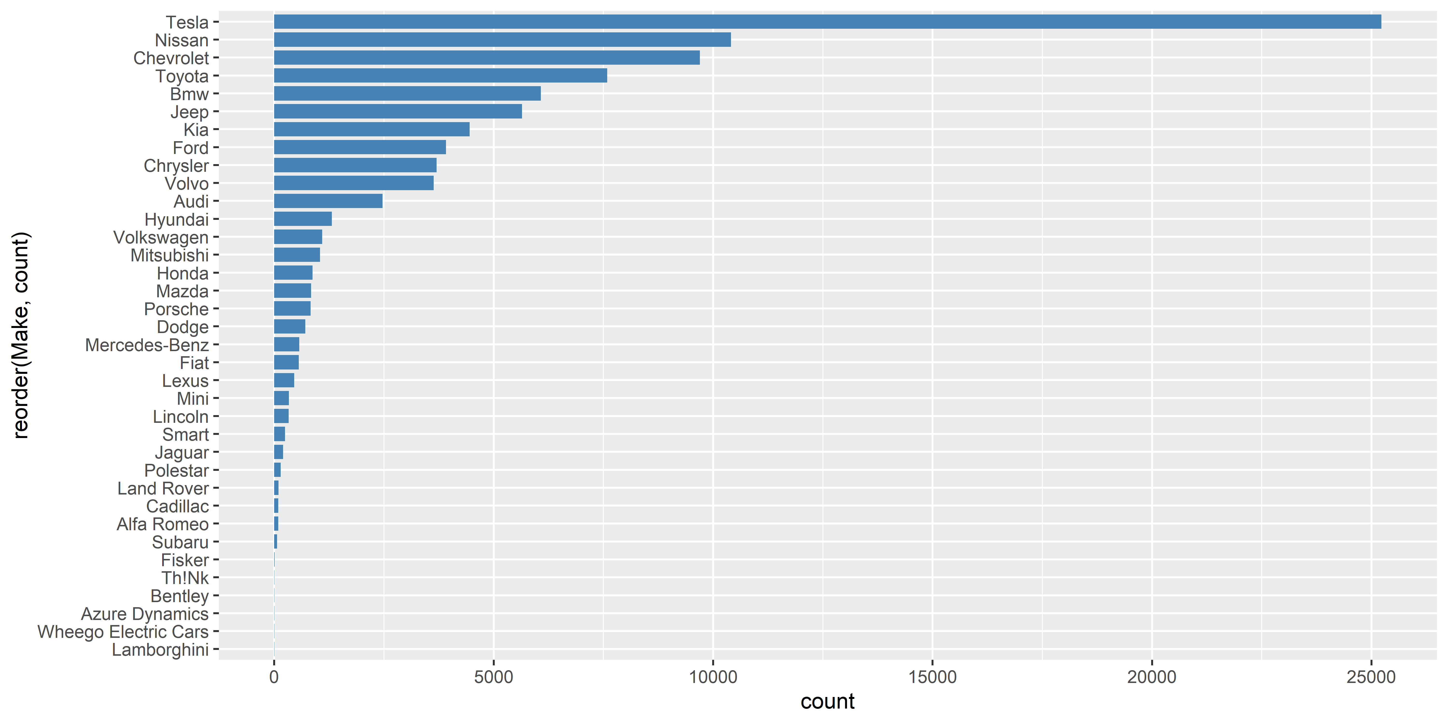

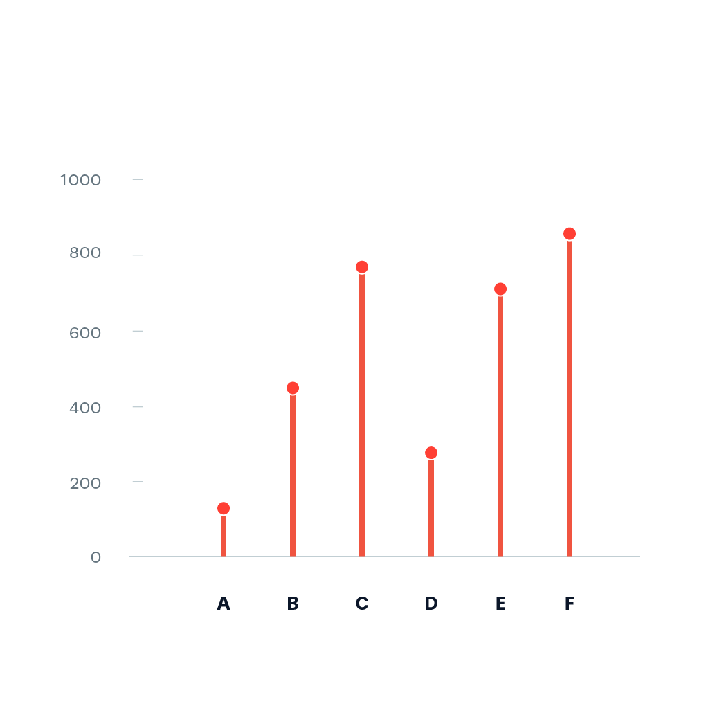
1.2 Lolipop Chart

Lolipop Chart adalah variasi bar chart yang menggunakan garis sebagai batang dan titik di ujungnya untuk menyoroti nilai kategori. Cocok digunakan saat bar chart terasa terlalu tebal atau ingin menampilkan data dengan lebih rapi. Karena tampilannya lebih elegan, lolipop chart sering dipakai dalam laporan atau presentasi, terutama untuk jumlah kategori yang tidak terlalu banyak.

Advanced

# Sort & Filter
data_ev_filtered <- data_ev %>%
  count(Make, name = "count") %>%
  dplyr::filter(count > 2000) %>%  
  arrange(desc(count)) %>%
  mutate(Make = str_to_title(Make))  

# Top 3
top3 <- head(data_ev_filtered$Make, 3)

chart <-
  ggplot(data_ev_filtered, aes(x = reorder(Make, count), y = count)) +
  
  # Lolipop Stick
  geom_segment(aes(xend = Make, y = 0, yend = count), 
               color = ifelse(data_ev_filtered$Make %in% top3, 
                              "steelblue", "gray50"),
               linewidth = 1.5) +
  
  # Lolipop Head
  geom_point(size = 10, 
             pch = 19, 
             color = ifelse(data_ev_filtered$Make %in% top3, 
                            "steelblue", "gray50")) +
  
  # Label
  geom_text(aes(label = count), color = "white", size = 2.5, fontface = "bold") +
  
  # Tema dan layout
  coord_flip() +
  theme_minimal() +
  scale_color_identity() +  # Apply warna tanpa legend
  geom_hline(yintercept = -0.3, color = "black", linewidth = 0.5) +  
  
  labs(title = "Dominasi tesla dalam pasar kendaraan listrik",
       subtitle = "Hanya menampilkan brand dengan lebih 2000 kendaraan terdaftar",
       x = "", 
       y = "") +
  
  theme(axis.text.y = element_text(size = 8, hjust = 1, face = "bold", 
                                   margin = margin(r = -25)),
        plot.title = element_text(hjust = -0.05, size = 14, face = "bold"),
        plot.subtitle = element_text(hjust = -0.04, size = 8),
        panel.grid.major.y = element_blank(),
        panel.grid.major.x = element_line(linetype = "dashed"),
        panel.grid.minor.x = element_line(linetype = "dashed")
  )

chart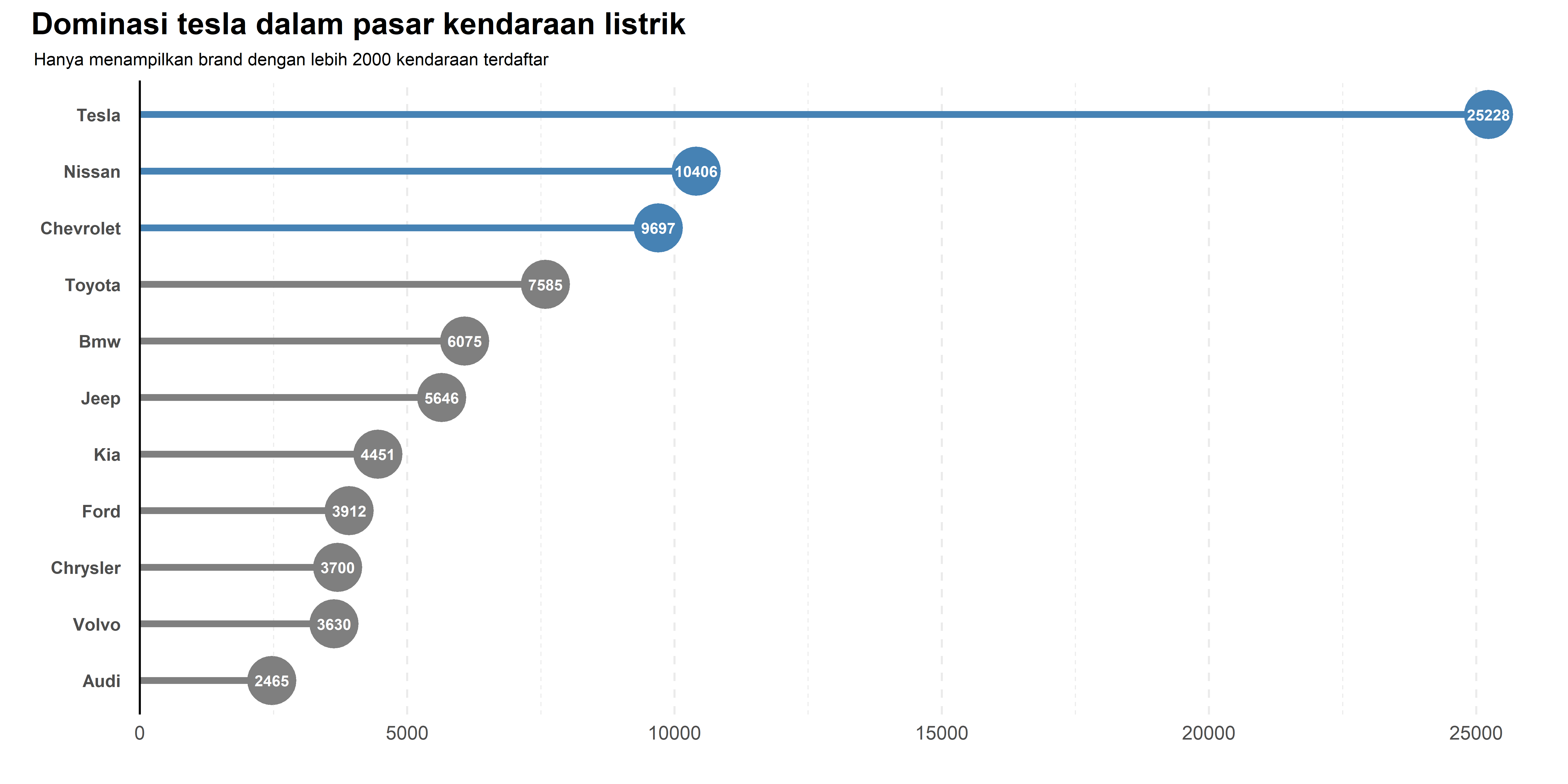

# Save Chart
ggsave("Chart/02_lolipop.png", chart, dpi = 300, height = 5, width = 10)

Meneruskan kustomisasi bar chart seperti highlight top 3, lolipop chart juga dapat digunakan untuk memberikan tampilan yang lebih bersih dan minimalis. Namun, karena kepala lolipop cukup besar, saya menyaring data dengan hanya menampilkan brand yang memiliki lebih dari 2000 kendaraan terdaftar agar visualisasi tetap jelas dan tidak terlalu ramai.

Size

chart <-
  ggplot(data_ev_filtered, aes(x = reorder(Make, count), y = count)) +
  
  # Lolipop Stick
  geom_segment(aes(xend = Make, y = 0, yend = count), 
               color = ifelse(data_ev_filtered$Make %in% top3, "steelblue", "gray50"),
               linewidth = 1.5) +
  
  # Lolipop Head 
  geom_point(aes(size = count, 
                 color = ifelse(Make %in% top3, "steelblue", "gray50")), 
             pch = 19) +
  
  # Tema dan layout
  coord_flip() +
  theme_minimal() +
  scale_color_identity() +  # Apply warna tanpa legend
  scale_size_continuous(range = c(2, 14)) +  # Ukuran lebih besar
  geom_hline(yintercept = -0.3, color = "black", linewidth = 0.5) +  
  
  labs(title = "Dominasi Tesla dalam Pasar Kendaraan Listrik",
       subtitle = "Hanya Menampilkan Brand dengan Lebih 2000 Kendaraan Terdaftar",
       x = "", 
       y = "") +
  
  theme(axis.text.y = element_text(size = 8, hjust = 1, face = "bold", 
                                   margin = margin(r = -25)),
        plot.title = element_text(hjust = -0.05, size = 14, face = "bold"),
        plot.subtitle = element_text(hjust = -0.04, size = 8),
        panel.grid.major.y = element_blank(),
        panel.grid.major.x = element_line(linetype = "dashed"),
        panel.grid.minor.x = element_line(linetype = "dashed"),
        legend.position = "none"
  )

chart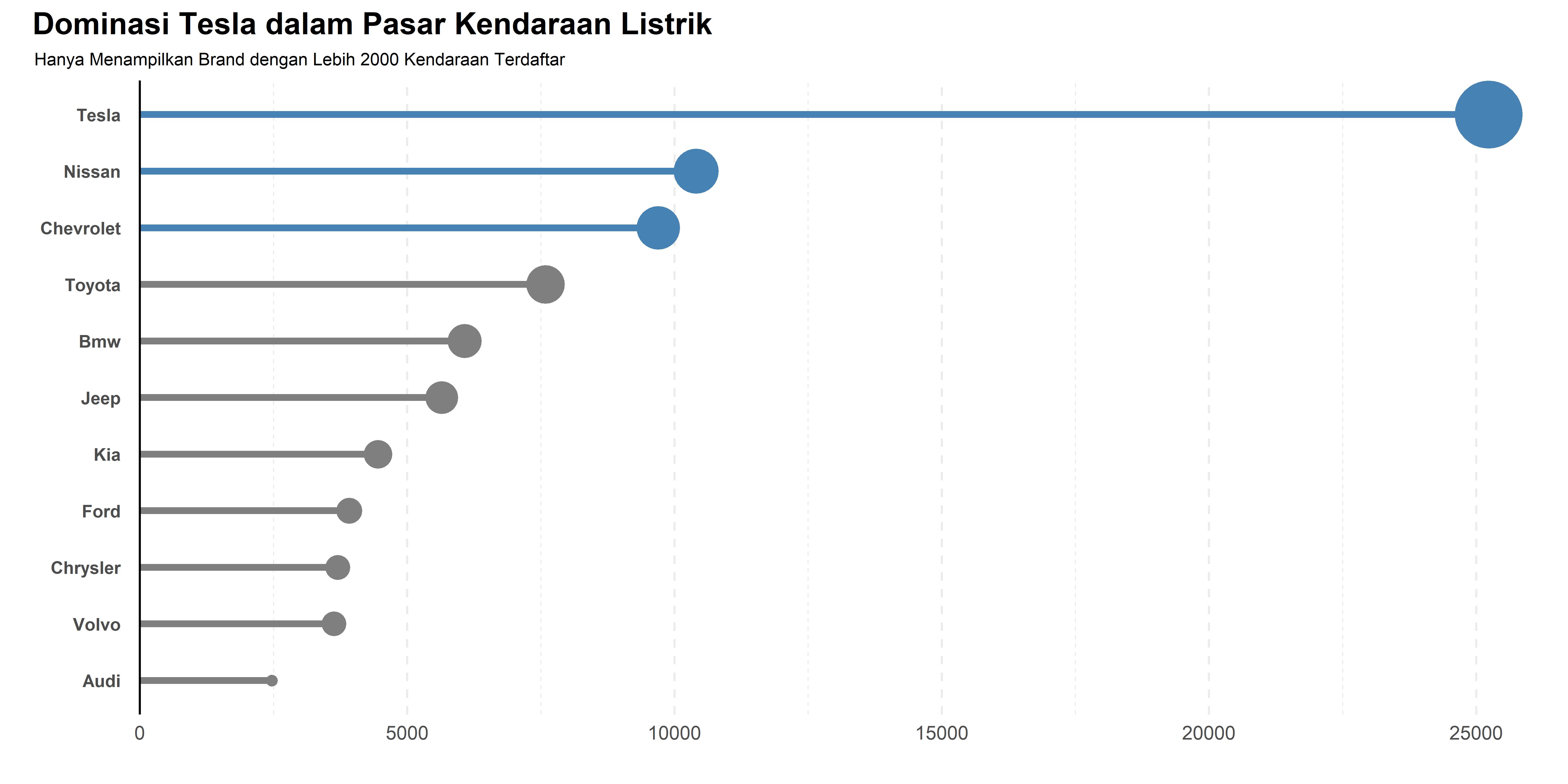

# Save Chart
ggsave("Chart/02_lolipop_var.png", chart, dpi = 300, height = 5, width = 10)

Selain itu, lolipop chart juga bisa dibuat dengan ukuran kepala yang bervariasi, mencerminkan jumlah kendaraan setiap brand. Namun, dalam kasus ini, saya menghapus label frekuensi di dalam lingkaran karena posisinya kurang pas untuk beberapa nilai.

Sederhana

chart <-
  ggplot(data_ev_filtered, aes(x = reorder(Make, count), y = count)) +
  
  # Lolipop Stick
  geom_segment(aes(xend = Make, y = 0, yend = count), 
               color = "steelblue",
               linewidth = 1.5) +
  
  # Lolipop Head 
  geom_point(size = 10, color = "steelblue", pch = 19) +
  coord_flip()

chart

Pondasi utama dari lolipop chart adalah geom_segment() yang membentuk garis sebagai batang lolipop dan geom_point() sebagai kepala lolipop.

1.3 Paired Bar

Paired Bar Chart digunakan untuk membandingkan dua kategori dalam satu variabel, misalnya jenis kendaraan listrik BEV vs PHEV atau kelayakan subsidi kendaraan. Dalam visualisasi ini, setiap merek memiliki dua batang berdampingan untuk menampilkan perbedaan jumlah pada setiap kategori.

Advanced 1

data_ev_grouped <- data_ev %>%
  count(Make, Electric.Vehicle.Type, name = "count") %>%
  dplyr::filter(count > 1000) %>%
  arrange(desc(count)) %>%
  mutate(Make = str_to_title(Make))  # Kapitalisasi merek

# Top 3 merek berdasarkan total kendaraan
top3 <- data_ev_grouped %>%
  group_by(Make) %>%
  summarise(total = sum(count)) %>%
  arrange(desc(total)) %>%
  head(3) %>%
  pull(Make)

# Paired Bar Chart
chart <- ggplot(data_ev_grouped, 
                aes(x = reorder(Make, count), y = count, fill = Electric.Vehicle.Type)) +
  
  # Bar chart dengan posisi dodge untuk perbandingan antar kategori
  geom_bar(stat = "identity", position = "dodge", width = 0.8) +
  
  # Label di ujung bar
  geom_text(aes(label = count), position = position_dodge(width = 0.8), 
            hjust = -0.2, size = 3) +
  
  # Garis grid horizontal
  geom_hline(yintercept = -0.3, color = "black", linewidth = 0.5) +
  
  coord_flip() +
  theme_minimal() +
  
  # Warna berbeda untuk kategori kendaraan listrik
  scale_fill_manual(values = c("BEV" = "#6a3f48",
                               "PHEV" = "#caa847")) +
  
  labs(title = "Dominasi Tesla dalam Pasar Kendaraan Listrik",
       subtitle = "Frekuensi Pendaftaran Kendaraan Listrik BEV dan PHEV dari Berbagai Merek",
       fill = "Jenis Kendaraan",  # Label legend
       x = "", 
       y = "") +
  
  theme(axis.text.y = element_text(size = 8, hjust = 1, face = "bold", 
                                   margin = margin(r = -25)),
        plot.title = element_text(hjust = -0.06, size = 14, face = "bold"),
        plot.subtitle = element_text(hjust = -0.05, size = 8),
        panel.grid.major.y = element_blank(),
        panel.grid.major.x = element_line(linetype = "dashed"),
        panel.grid.minor.x = element_line(linetype = "dashed"),
        legend.text = element_text(size = 8),  
        legend.title = element_text(size = 8), 
        legend.key.size = unit(0.5, "cm")     
  )

chart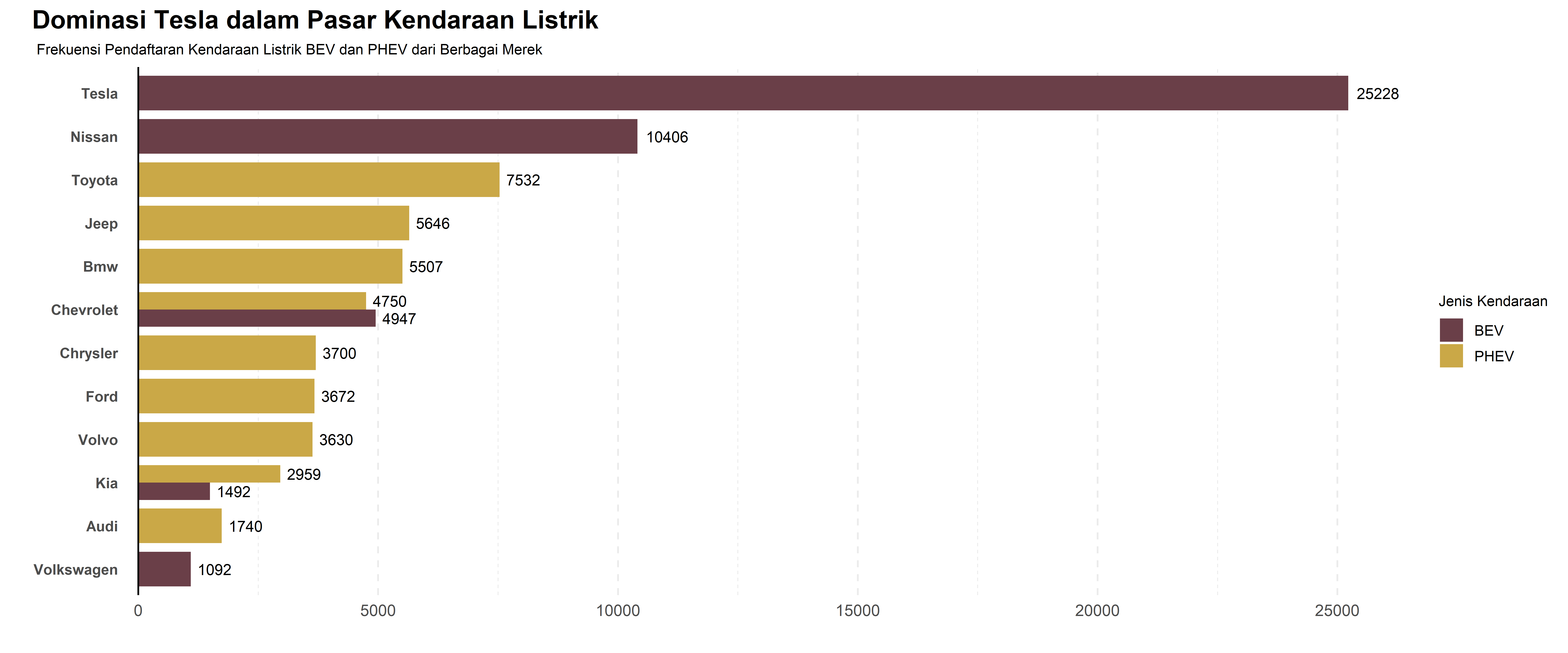

# Save Chart
ggsave("Chart/01_Bar_Paired.png", chart, dpi = 300, height = 5, width = 10)

Pada contoh ini, saya hanya menampilkan merek dengan lebih dari 1000 kendaraan terdaftar untuk menjaga visualisasi tetap fokus dan mudah dibaca. Warna berbeda digunakan untuk membedakan kategori, sehingga lebih jelas dalam melihat dominasi masing-masing jenis kendaraan dalam satu merek. Tesla masih mendominasi pasar EV, terutama dalam kategori BEV, sementara merek lain seperti Toyota dan Jeep lebih banyak dalam kategori PHEV.

Advanced 2

data_ev_grouped <- data_ev %>%
  count(Make, CAFV.Eligibility.Simple, name = "count") %>%
  dplyr::filter(count > 1000) %>%
  arrange(desc(count)) %>%
  mutate(Make = str_to_title(Make))  # Kapitalisasi merek

# Top 3 merek berdasarkan total kendaraan
top3 <- data_ev_grouped %>%
  group_by(Make) %>%
  summarise(total = sum(count)) %>%
  arrange(desc(total)) %>%
  head(3) %>%
  pull(Make)

# Paired Bar Chart
chart <- ggplot(data_ev_grouped, 
                aes(x = reorder(Make, count), y = count, fill = CAFV.Eligibility.Simple)) +
  
  # Bar chart dengan posisi dodge untuk perbandingan antar kategori
  geom_bar(stat = "identity", position = "dodge", width = 0.8) +
  
  # Label di ujung bar
  geom_text(aes(label = count), position = position_dodge(width = 0.8), 
            hjust = -0.2, size = 3) +
  
  # Garis grid horizontal
  geom_hline(yintercept = -0.3, color = "black", linewidth = 0.5) +
  
  coord_flip() +
  theme_minimal() +
  
  # Warna berbeda untuk kategori kendaraan listrik
  scale_fill_manual(values = c("Eligible" = "#88b07e",
                               "Not Eligible" = "#9c3b66")) +
  
  labs(title = "Dominasi Tesla dalam Pasar Kendaraan Listrik",
       subtitle = "Perbandingan Kelayakan Kendaraan Listrik di Berbagai Merek",
       fill = "Jenis Kendaraan",  # Label legend
       x = "", 
       y = "") +
  
  theme(axis.text.y = element_text(size = 8, hjust = 1, face = "bold", 
                                   margin = margin(r = -25)),
        plot.title = element_text(hjust = -0.06, size = 14, face = "bold"),
        plot.subtitle = element_text(hjust = -0.05, size = 8),
        panel.grid.major.y = element_blank(),
        panel.grid.major.x = element_line(linetype = "dashed"),
        panel.grid.minor.x = element_line(linetype = "dashed"),
        legend.text = element_text(size = 8),  
        legend.title = element_text(size = 8), 
        legend.key.size = unit(0.5, "cm")     
  )

chart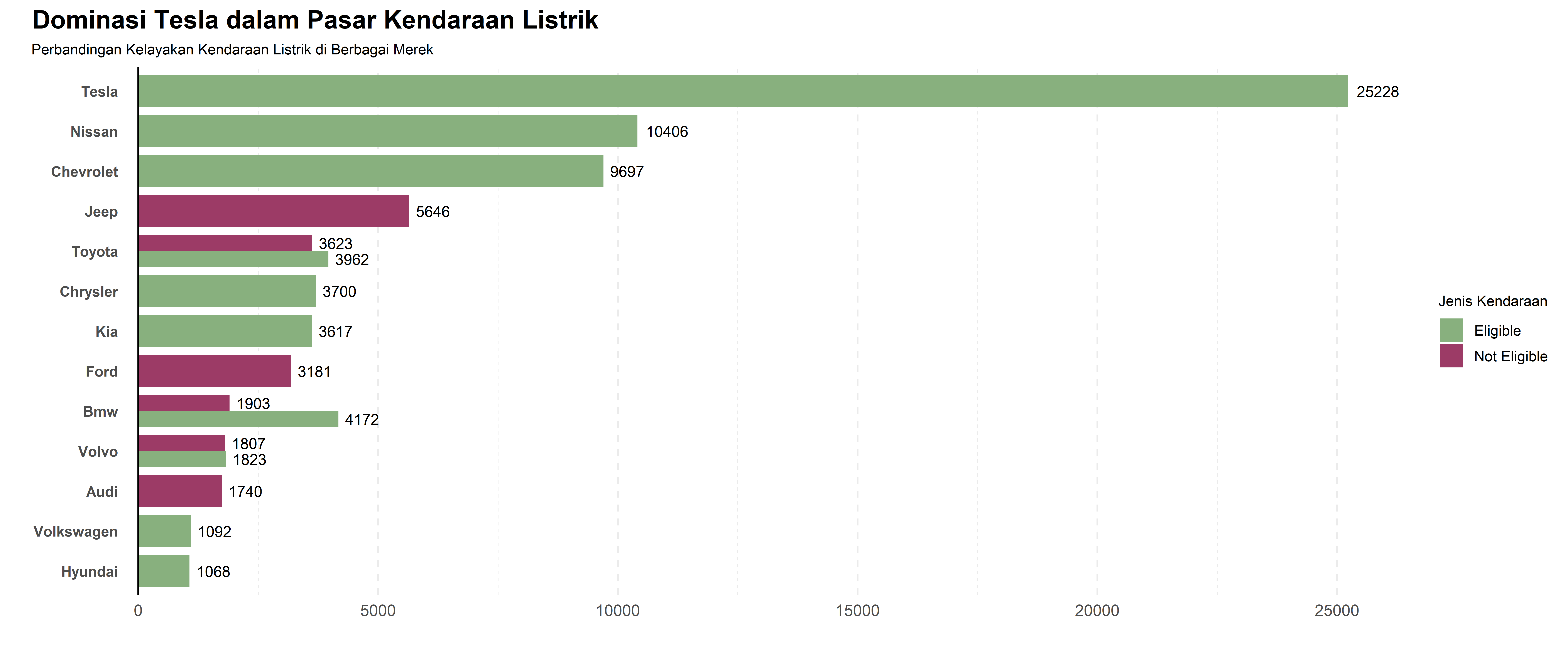

# Save Chart
ggsave("Chart/01_Bar_Paired.png", chart, dpi = 300, height = 5, width = 10)

Grafik Paired Bar Chart ini membandingkan kelayakan kendaraan listrik dari berbagai merek, dibagi menjadi dua kategori: “Eligible” (layak mendapatkan subsidi atau insentif) dan “Not Eligible” (tidak layak mendapatkan subsidi).

Dari hasil visualisasi, Tesla masih menjadi pemimpin dengan mayoritas kendaraannya termasuk dalam kategori “Eligible”, menunjukkan bahwa banyak model Tesla memenuhi syarat untuk subsidi atau program insentif kendaraan listrik. Di sisi lain, beberapa merek seperti Jeep dan Ford memiliki jumlah kendaraan “Not Eligible” yang cukup besar, menunjukkan bahwa banyak model mereka tidak memenuhi syarat yang ditetapkan.

Sederhana

ggplot(data_ev, 
       aes(x = Make, fill=Electric.Vehicle.Type)) +
  # Bar chart
  geom_bar(position="dodge") +
  coord_flip()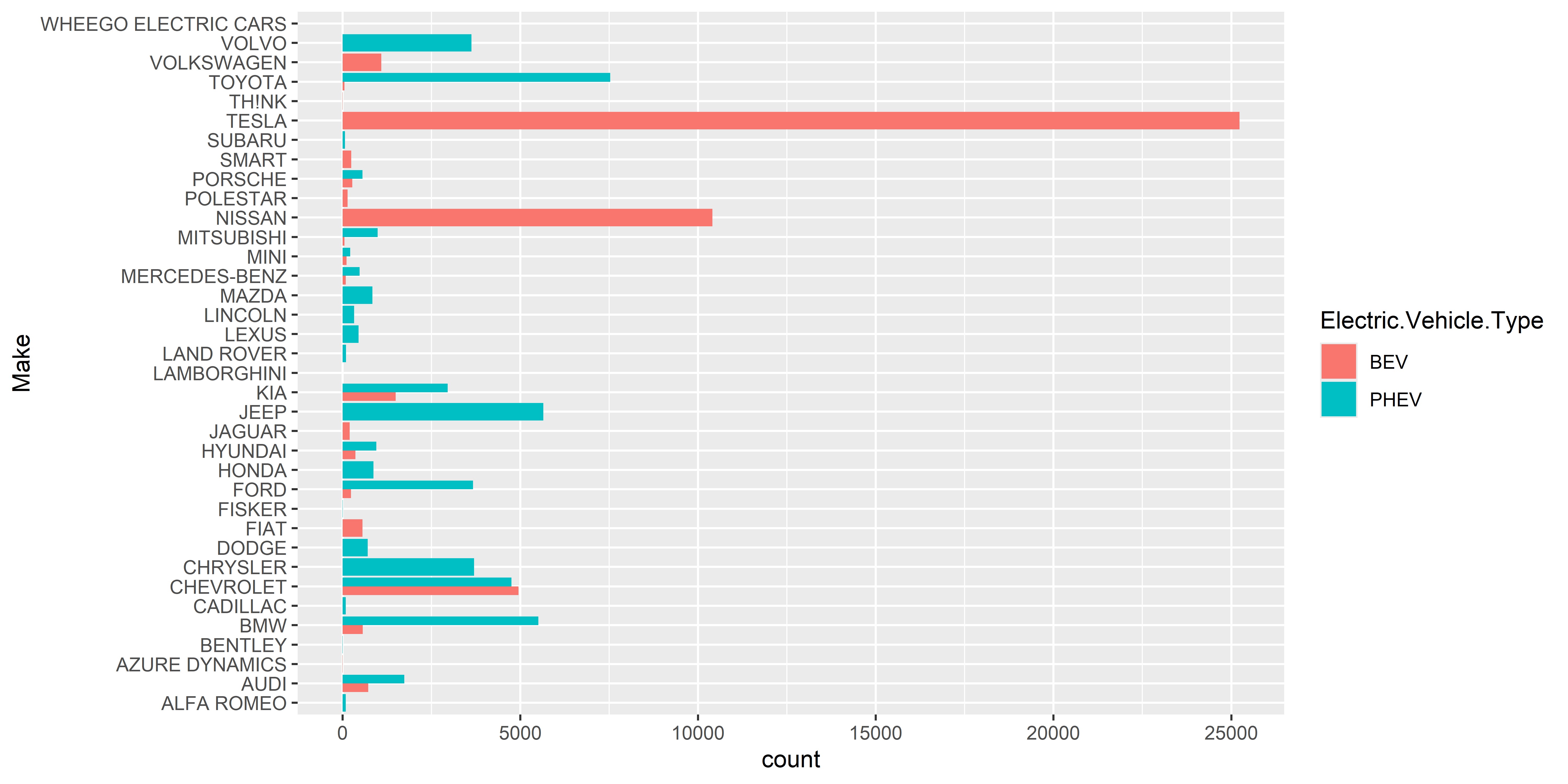

Pondasi utama dari paired bar chart dalam ggplot2 adalah geom_bar(position = "dodge"), yang memastikan kedua kategori tampil bersebelahan dalam satu sumbu. Variasi ini cocok digunakan ketika ingin menganalisis perbandingan kategori dalam satu kelompok, seperti jenis kendaraan, status kelayakan, atau perbedaan regional.

1.4 Stacked Bar

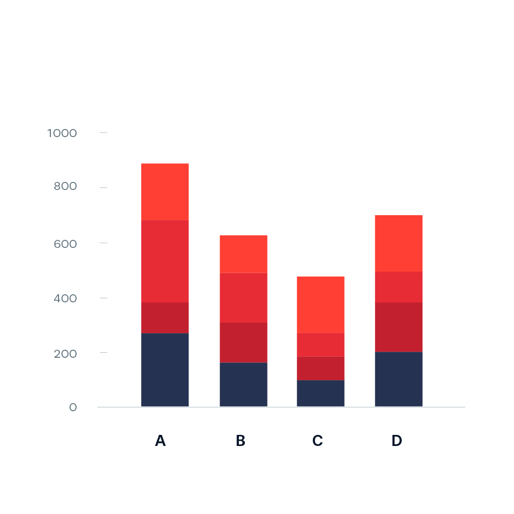
Menampilkan perbandingan komposisi antar kategori.

Advanced Freq

data_ev_grouped <- data_ev %>%
  count(Make, CAFV.Eligibility.Simple, name = "count") %>%
  dplyr::filter(count > 1000) %>%
  arrange(desc(count)) %>%
  mutate(Make = str_to_title(Make))  # Kapitalisasi merek

# Top 3 merek berdasarkan total kendaraan
top3 <- data_ev_grouped %>%
  group_by(Make) %>%
  summarise(total = sum(count)) %>%
  arrange(desc(total)) %>%
  head(3) %>%
  pull(Make)

# Paired Bar Chart
chart <- ggplot(data_ev_grouped, 
                aes(x = reorder(Make, count), y = count, fill = CAFV.Eligibility.Simple)) +
  
  # Bar chart dengan posisi dodge untuk perbandingan antar kategori
  geom_bar(stat = "identity", position = "stack", width = 0.8) +
  
  # Label di ujung bar
  geom_text(aes(label = count), 
            position = position_stack(vjust = 0.5), 
            size = 3, color = "white", fontface = "bold") +
  
  # Garis grid horizontal
  geom_hline(yintercept = -0.3, color = "black", linewidth = 0.5) +
  
  coord_flip() +
  theme_minimal() +
  
  # Warna berbeda untuk kategori kendaraan listrik
  scale_fill_manual(values = c("Eligible" = "#88b07e",
                               "Not Eligible" = "#9c3b66")) +
  
  labs(title = "Dominasi Tesla dalam Pasar Kendaraan Listrik",
       subtitle = "Perbandingan Kelayakan Kendaraan Listrik di Berbagai Merek",
       fill = "Jenis Kendaraan",  # Label legend
       x = "", 
       y = "") +
  
  theme(axis.text.y = element_text(size = 8, hjust = 1, face = "bold", 
                                   margin = margin(r = -25)),
        plot.title = element_text(hjust = -0.06, size = 14, face = "bold"),
        plot.subtitle = element_text(hjust = -0.05, size = 8),
        panel.grid.major.y = element_blank(),
        panel.grid.major.x = element_line(linetype = "dashed"),
        panel.grid.minor.x = element_line(linetype = "dashed"),
        legend.text = element_text(size = 8),  
        legend.title = element_text(size = 8), 
        legend.key.size = unit(0.5, "cm")     
  )

chart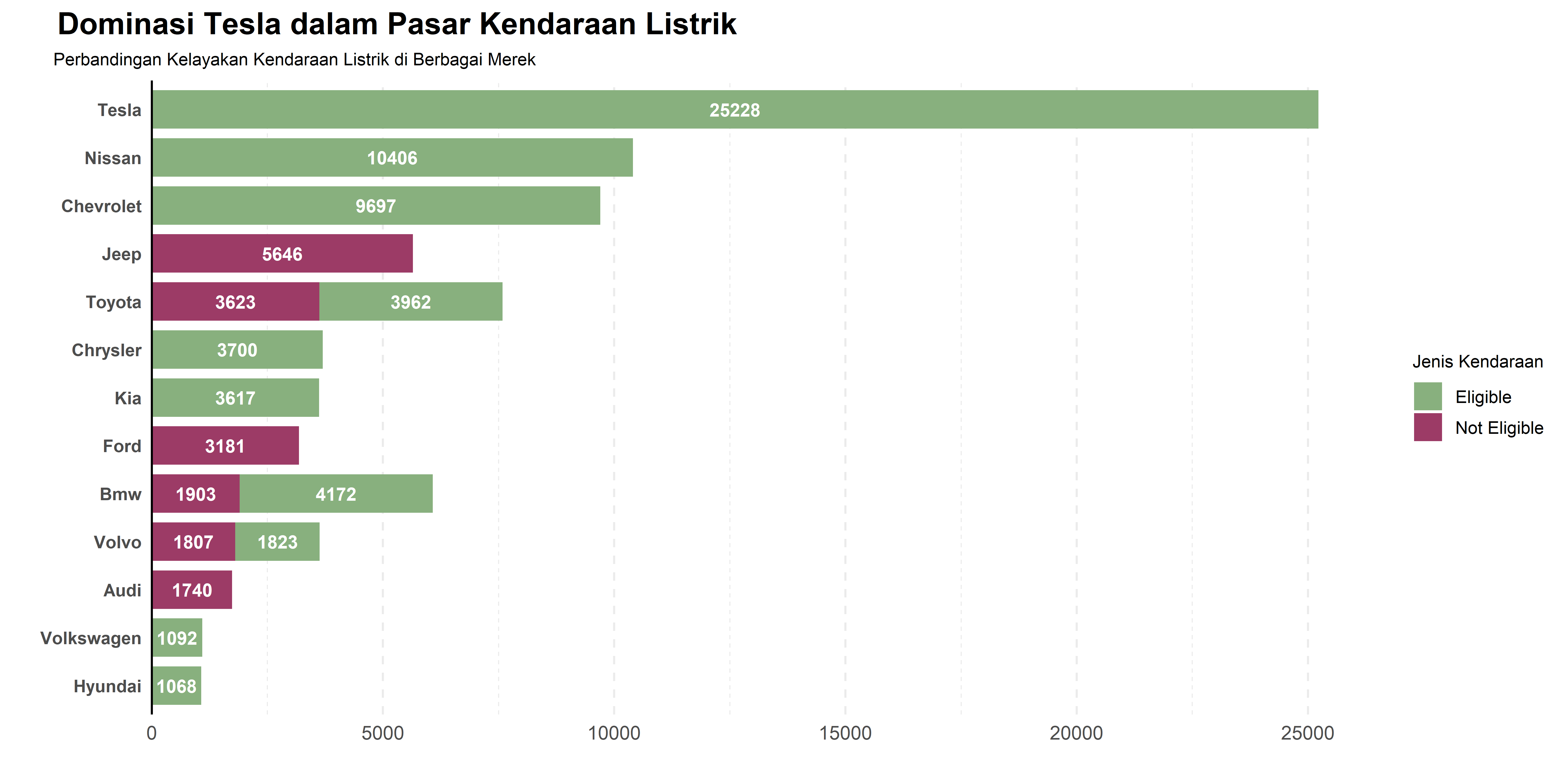

# Save Chart
ggsave("Chart/01_Bar_Paired.png", chart, dpi = 300, height = 5, width = 10)

Advanced %

data_ev_grouped <- data_ev %>%
  count(Make, CAFV.Eligibility.Simple, name = "count") %>%
  dplyr::filter(sum(count) > 1000, .by = Make) %>%  # Pastikan hanya merek dengan total >1000 kendaraan
  arrange(desc(count)) %>%
  mutate(Make = str_to_title(Make))  # Kapitalisasi merek

# Hitung proporsi dalam setiap merek
data_ev_grouped <- data_ev_grouped %>%
  group_by(Make) %>%
  mutate(percentage = count / sum(count)) %>%
  ungroup()

# Stacked Bar Chart dengan Persentase
chart <- ggplot(data_ev_grouped, 
                aes(x = Make, y = percentage, fill = CAFV.Eligibility.Simple)) +
  
  # Bar chart full persentase
  geom_bar(stat = "identity", position = "fill", width = 0.8) +
  
  # Label di tengah bar dalam format persen
  geom_text(aes(label = scales::percent(percentage, accuracy = 1)), 
            position = position_fill(vjust = 0.5), 
            size = 3, color = "white", fontface = "bold") +
  
  # Grid horizontal
  geom_hline(yintercept = 0, color = "black", linewidth = 0.5) +
  
  coord_flip() +
  theme_minimal() +
  
  # Warna berbeda untuk kategori eligibility
  scale_fill_manual(values = c("Not Eligible" = "#9c3b66",
                               "Eligible" = "#88b07e")) +
  
  labs(title = "Dominasi Tesla dalam Pasar Kendaraan Listrik",
       subtitle = "Distribusi Persentase Kelayakan Kendaraan Listrik di Berbagai Merek",
       fill = "Jenis Kendaraan",
       x = "", 
       y = "Persentase") +
  
  scale_y_continuous(labels = scales::percent_format(accuracy = 1)) +  # Pastikan sumbu Y dalam persen
  
  theme(axis.text.y = element_text(size = 8, hjust = 1, face = "bold", 
                                   margin = margin(r = -25)),
        plot.title = element_text(hjust = -0.07, size = 14, face = "bold"),
        plot.subtitle = element_text(hjust = -0.06, size = 8),
        panel.grid.major.y = element_blank(),
        panel.grid.major.x = element_line(linetype = "dashed"),
        panel.grid.minor.x = element_line(linetype = "dashed"),
        legend.text = element_text(size = 8),  
        legend.key.size = unit(0.5, "cm"),
        legend.position = "top",
        legend.direction = "horizontal",
        legend.justification = c(-0.055, 0.5)
  ) +
  guides(fill = guide_legend(title = NULL))

chart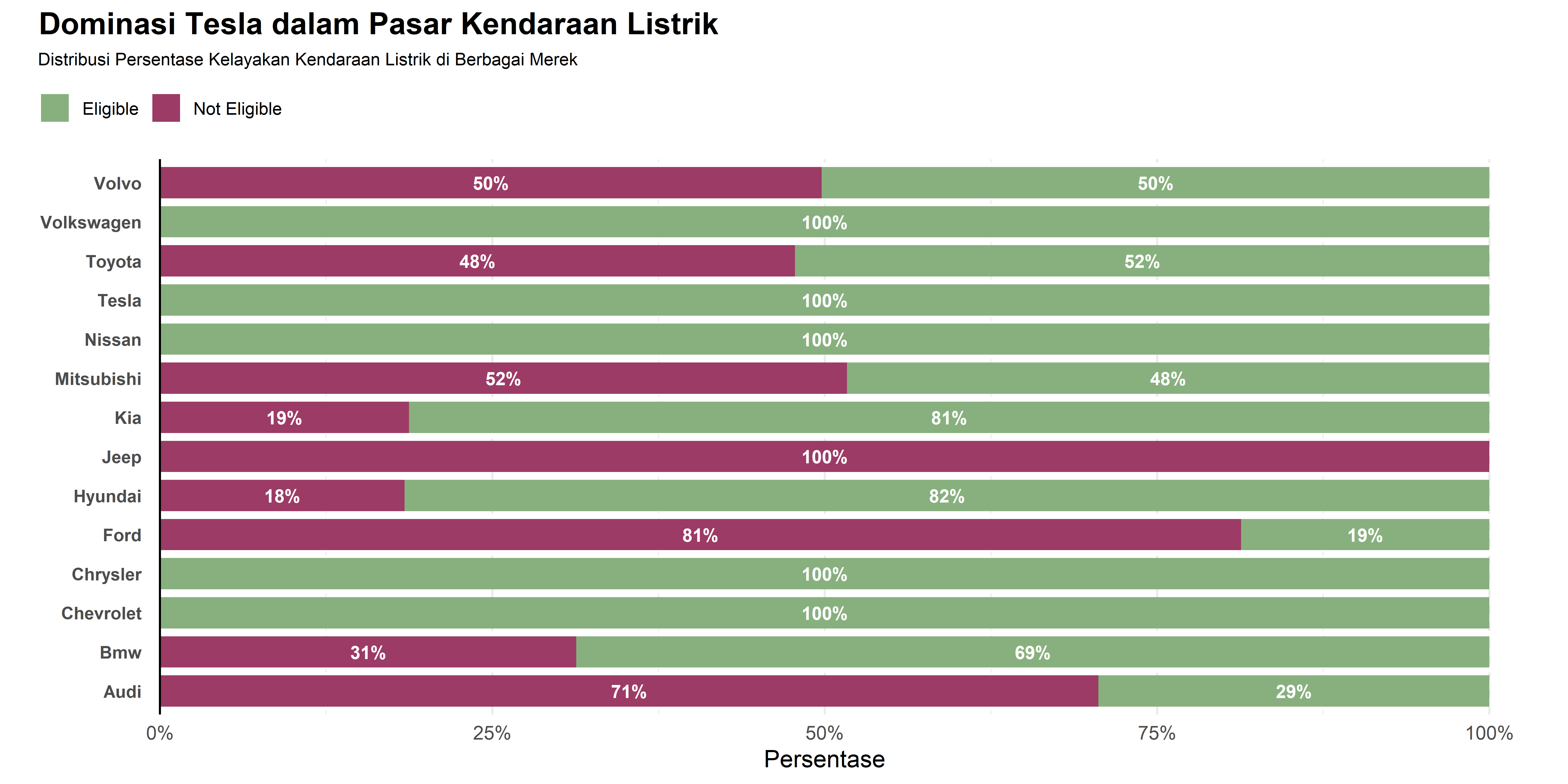

# Save Chart
ggsave("Chart/Stacked_Bar_Percentage.png", chart, dpi = 300, height = 5, width = 10)

Sederhana

ggplot(data_ev, 
       aes(x = Make, fill=Electric.Vehicle.Type)) +
  # Bar chart
  geom_bar(position="stack") +
  coord_flip()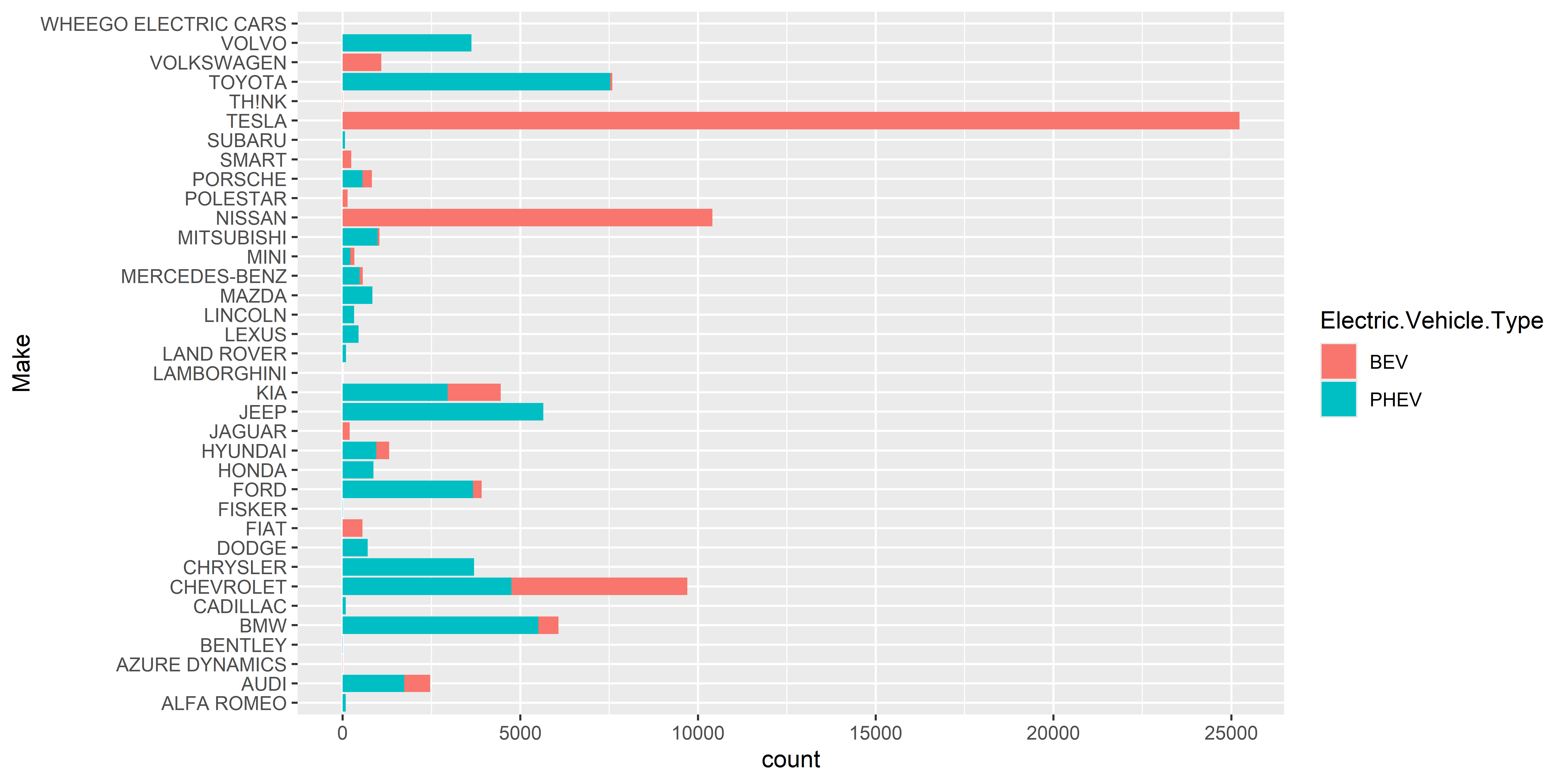

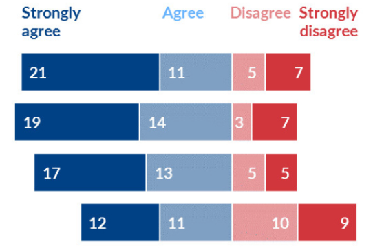
1.5 Diverging Bar

Menunjukkan distribusi kategori dengan skala positif-negatif.

# Buat mapping unik untuk setiap pertanyaan
question_map <- data_survey %>%
  distinct(Question) %>%
  mutate(Q_Label = paste0("Q.", str_pad(row_number(), 2, pad = "0")))  # Ubah ke dua digit

# Gabungkan kembali ke data asli
data_survey <- data_survey %>%
  left_join(question_map, by = "Question") %>%
  select(-Question) %>%
  rename(Question = Q_Label)  # Ganti dengan label baru

# Konversi teks ke angka menggunakan mutate + case_when()
data_survey_cleaned <- data_survey %>%
  
  # Filter hanya respon valid (hapus Not Applicable dan data kosong)
  dplyr::filter(Response.Text != "Not Applicable", Response.Text != "") %>%
  
  # Ubah Response.Text menjadi angka
  mutate(Response.Value = case_when(
    Response.Text == "Strongly Agree" ~ 2,
    Response.Text == "Agree" ~ 1,
    Response.Text == "Disagree" ~ -1,
    Response.Text == "Strongly Disagree" ~ -2
  )) %>%
  
  # Hitung jumlah masing-masing respons per pertanyaan
  count(Question, Response.Text, Response.Value, name = "Count")

# Pastikan faktor dalam urutan yang benar
data_survey_cleaned <- data_survey_cleaned %>%
  mutate(Response.Text = factor(Response.Text, 
                                levels = c("Strongly Agree", "Agree", "Disagree", "Strongly Disagree")))

# Ubah sisi negatif untuk visualisasi divergen
data_survey_cleaned <- data_survey_cleaned %>%
  mutate(Count = ifelse(Response.Value < 0, -Count, Count)) %>%
  dplyr::filter(Question != "Q.12") %>%
  mutate(Question = factor(Question, levels = rev(unique(Question))))

# Warna divergen
color_palette <- c("Strongly Agree" = "#08306b",
                   "Agree" = "#6baed6",
                   "Disagree" = "#fcae91",
                   "Strongly Disagree" = "#cb181d")

# Plot diverging bar chart dengan label frekuensi
ggplot(data_survey_cleaned, aes(x = Question, y = Count, fill = Response.Text)) +
  geom_bar(stat = "identity", position = "stack", width = 0.8) +
  scale_fill_manual(values = color_palette) +
  
  # Tambahkan label frekuensi di dalam bar
  geom_text(aes(label = abs(Count)), 
            position = position_stack(vjust = 0.5), 
            size = 3, color = "white", fontface = "bold") +

  coord_flip() +
  theme_minimal() +
  
  labs(title = "Survey Responses - Diverging Bar Chart",
       subtitle = "Distribusi Sentimen Responden Berdasarkan Pertanyaan",
       x = "", 
       y = "") +
  
  scale_y_continuous(breaks = seq(-50, 50, 10), labels = abs(seq(-50, 50, 10))) +  # Pastikan label y tetap positif
  theme(panel.grid.major.y = element_blank(),
        panel.grid.minor.y = element_blank(),
        panel.grid.major.x = element_line(linetype = "dashed"),
        legend.position = "top",
        legend.direction = "horizontal",
        legend.title = element_blank())  # Hilangkan judul legend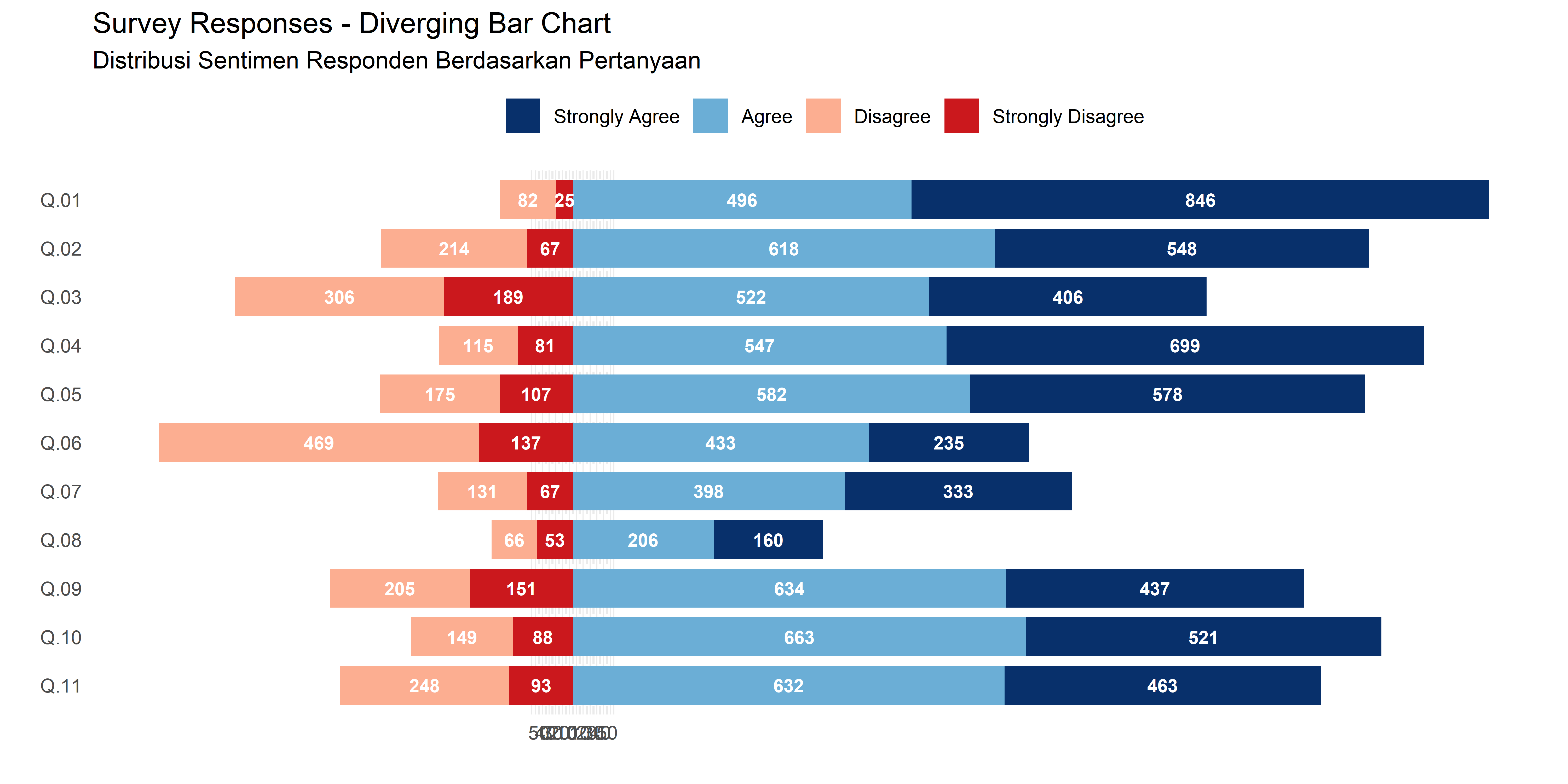

1.6 Dot Plot

Digunakan untuk menunjukkan distribusi atau perbandingan antar kategori.

# Buat dataset PISA
data_pisa <- data.frame(
  Country = c("Japan", "Switzerland", "Denmark", "France", "Australia", 
              "United States", "Turkey", "Greece", "Chile", "Mexico"),
  Math = c(532, 520, 509, 495, 503, 487, 454, 437, 423, 408), 
  Reading = c(520, 506, 497, 493, 499, 480, 460, 440, 420, 405)
)

# Ubah data ke format long untuk visualisasi dot plot
data_pisa_long <- data_pisa %>%
  pivot_longer(cols = c(Math, Reading), names_to = "Subject", values_to = "Score")

# Warna untuk kategori Math dan Reading
color_palette <- c("Math" = "#1f77b4", "Reading" = "#d62728")

# Plot dot plot
ggplot(data_pisa_long, aes(x = Score, y = reorder(Country, Score), color = Subject)) +
  geom_point(size = 4) +  # Titik
  geom_line(aes(group = Country), color = "black") +  # Garis penghubung antara dua titik
  scale_color_manual(values = color_palette) +  # Warna kategori
  theme_minimal() +
  labs(title = "PISA Scores for Math and Reading among 10 OECD Countries",
       x = "PISA Score",
       y = "",
       color = "Subject") +
  theme(legend.position = "top",
        legend.direction = "horizontal",
        plot.title = element_text(size = 14, face = "bold"),
        axis.text.y = element_text(face = "bold"))

1.7 Marimekko and Mosaic Charts

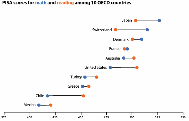
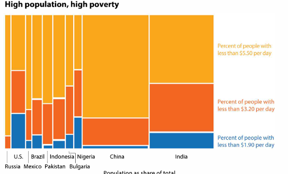
Visualisasi untuk membandingkan proporsi dua variabel kategori.

1.8 Unit, Isotype, and Waffle Charts

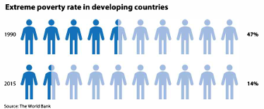
Digunakan untuk menampilkan proporsi dalam bentuk ikon atau blok.

1.8.1 Unit Chart

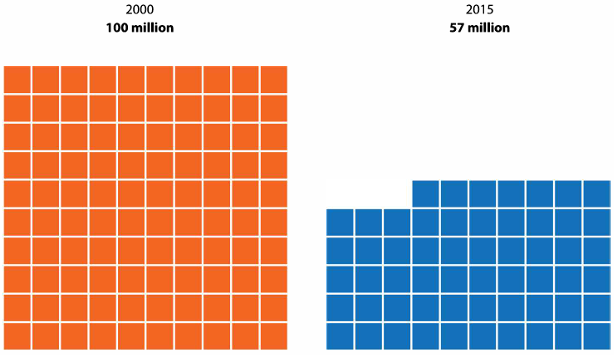
# Buat dataset grid untuk tahun 2000 (100 kotak) dan tahun 2015 (57 kotak)
unit_2000 <- expand.grid(x = 1:10, y = 1:10) %>% 
  mutate(Year = "2000") %>% 
  slice(1:100)  # Ambil hanya 100 unit

unit_2015 <- expand.grid(x = 1:10, y = 1:10) %>% 
  mutate(Year = "2015") %>% 
  slice(1:57)  # Ambil hanya 57 unit

# Gabungkan dataset
unit_chart_data <- bind_rows(unit_2000, unit_2015)

# Plot Unit Chart
ggplot(unit_chart_data, aes(x = x, y = y, fill = Year)) +
  geom_tile(color = "white", linewidth = 0.5) +
  scale_fill_manual(values = c("2000" = "orange", "2015" = "blue")) +
  labs(title = "Unit Chart: Poverty Reduction",
       subtitle = "Each square represents 1 million people",
       x = "", y = "") +
  facet_wrap(~Year, scales = "free") +  # Pisahkan per Tahun
  theme_void() +
  theme(legend.position = "none")  # Sembunyikan legend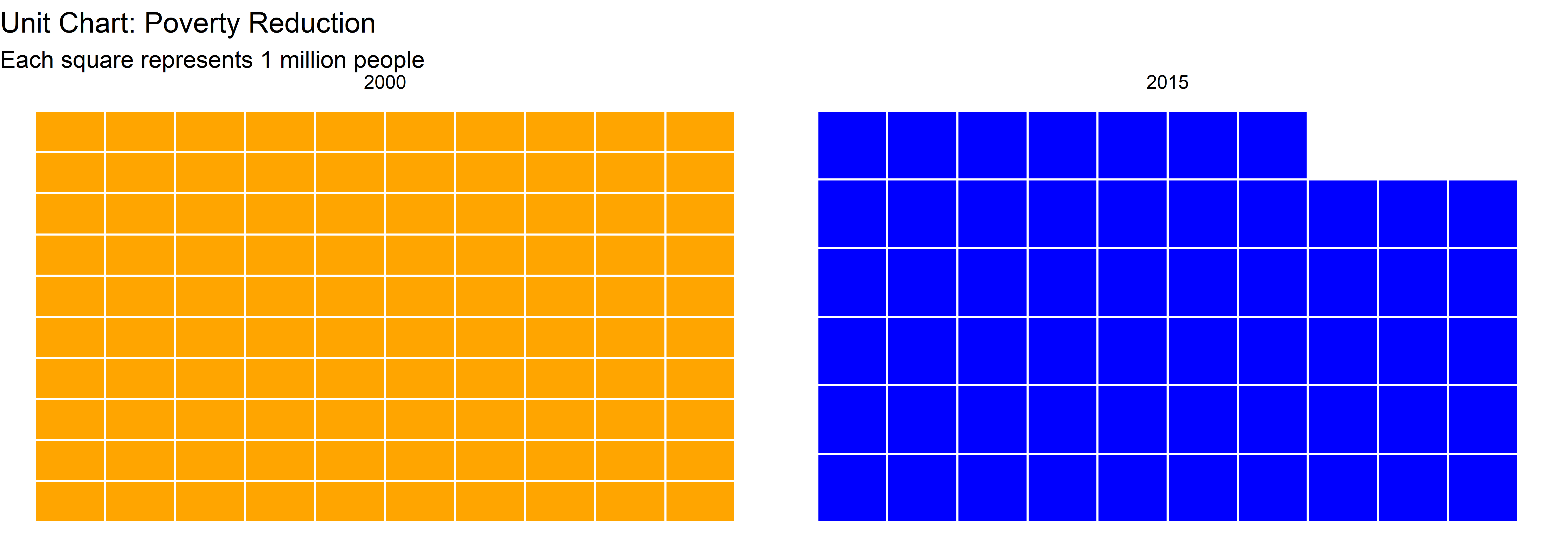

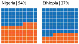
1.8.2 Waffle Chart

# Buat data proporsi
poverty_data <- c("Nigeria (54%)" = 54, "Ethiopia (27%)" = 27, "Others" = 19)

# Waffle Chart
waffle(poverty_data, rows = 10, colors = c("#E15759", "#F28E2B", "#BAB0AC")) +
  labs(title = "Waffle Chart: Poverty Distribution",
       subtitle = "Percentage of People in Extreme Poverty") +
  theme_minimal()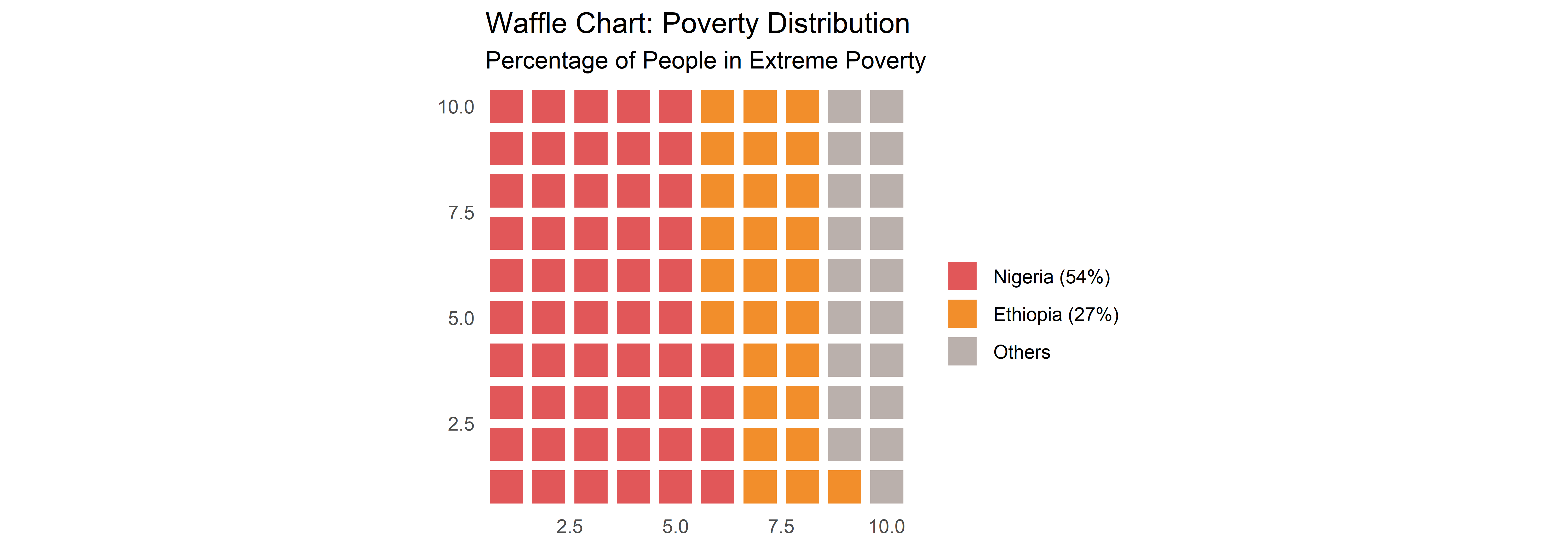

1.9 Heatmap

Visualisasi matriks yang menggunakan warna untuk mewakili nilai numerik.

# Membuat data untuk 3 bulan (Januari-Maret 2024)
dates <- seq(as.Date("2024-01-01"), as.Date("2024-03-31"), by = "day")
set.seed(123)
data <- data.frame(
  date = dates,
  value = runif(length(dates), 0, 100)
)

# Menambahkan informasi hari dan minggu
data <- data %>%
  mutate(
    weekday = wday(date, week_start = 1), # 1 = Senin sebagai awal minggu
    week = week(date),
    month = format(date, "%B"),
    monthweek = as.numeric(format(date, "%W")) - 
                as.numeric(format(as.Date(paste0(format(date, "%Y-%m"), "-01")), "%W")) + 1
  )

# Membuat plot
ggplot(data, aes(x = weekday, y = monthweek, fill = value)) +
  geom_tile(color = "white", size = 0.1) +
  scale_fill_gradient(low = "#e5f5f9", high = "#2ca25f") +
  facet_wrap(~month, ncol = 3, scales = "free") +
  scale_x_continuous(
    breaks = 1:7,
    labels = c("Su", "Mo", "Tu", "We", "Th", "Fr", "Sa"),
    expand = c(0, 0)
  ) +
  scale_y_reverse(expand = c(0, 0)) +
  theme_minimal() +
  theme(
    axis.title = element_blank(),
    panel.grid = element_blank(),
    legend.position = "none",
    strip.text = element_text(size = 12, face = "bold"),
    plot.background = element_rect(fill = "white", color = NA),
    panel.background = element_rect(fill = "white", color = NA)
  ) +
  labs(title = "Calendar Heatmap")

Warning: Using `size` aesthetic for lines was deprecated in ggplot2 3.4.0.
ℹ Please use `linewidth` instead.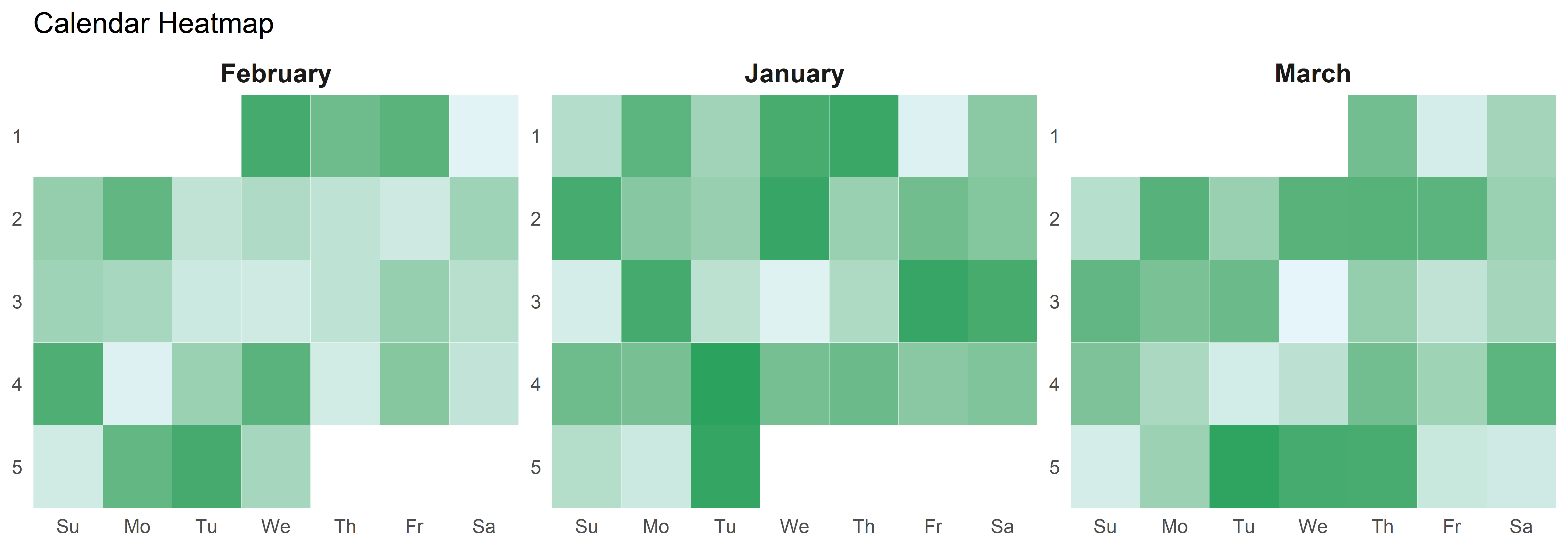

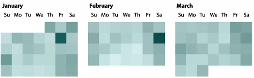
# Alternative menggunakan package calendR
# Membuat tiga kalender terpisah
calendR(year = 2024, month = 1, 
        special.days = runif(31, 0, 100),
        gradient = TRUE,
        low.col = "#e5f5f9",
        special.col = "#2ca25f",
        title = "January 2024")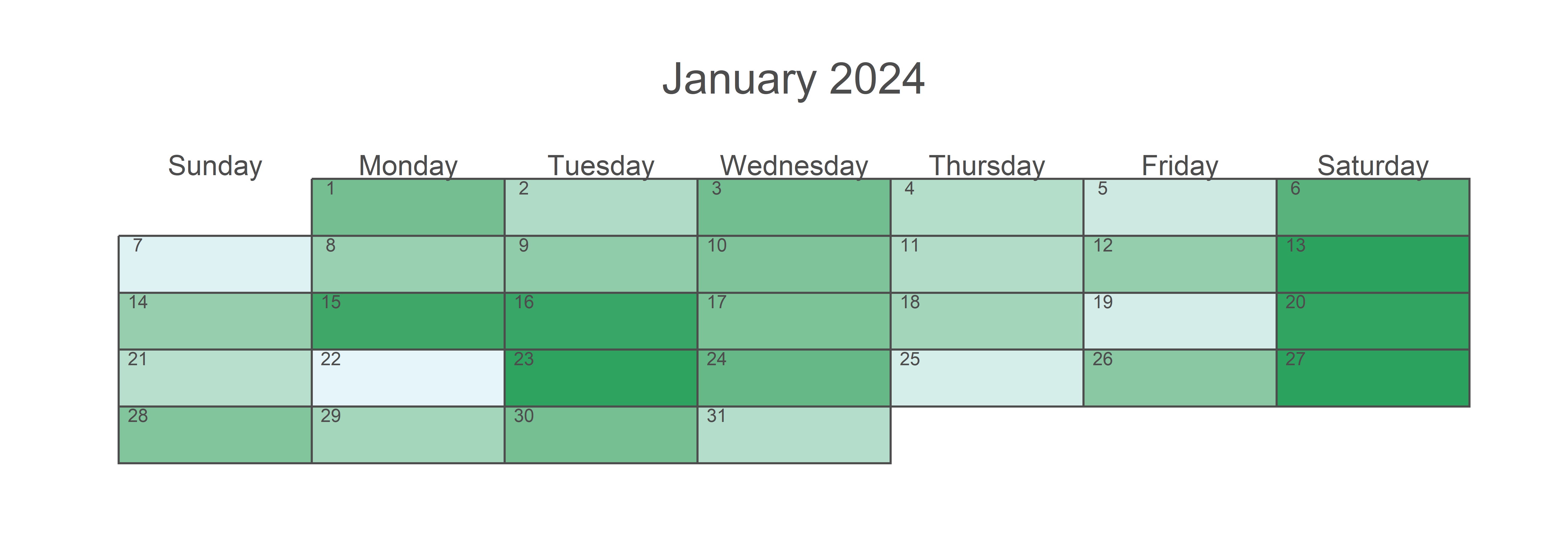

calendR(year = 2024, month = 2, 
        special.days = runif(29, 0, 100),
        gradient = TRUE,
        low.col = "#e5f5f9",
        special.col = "#2ca25f",
        title = "February 2024")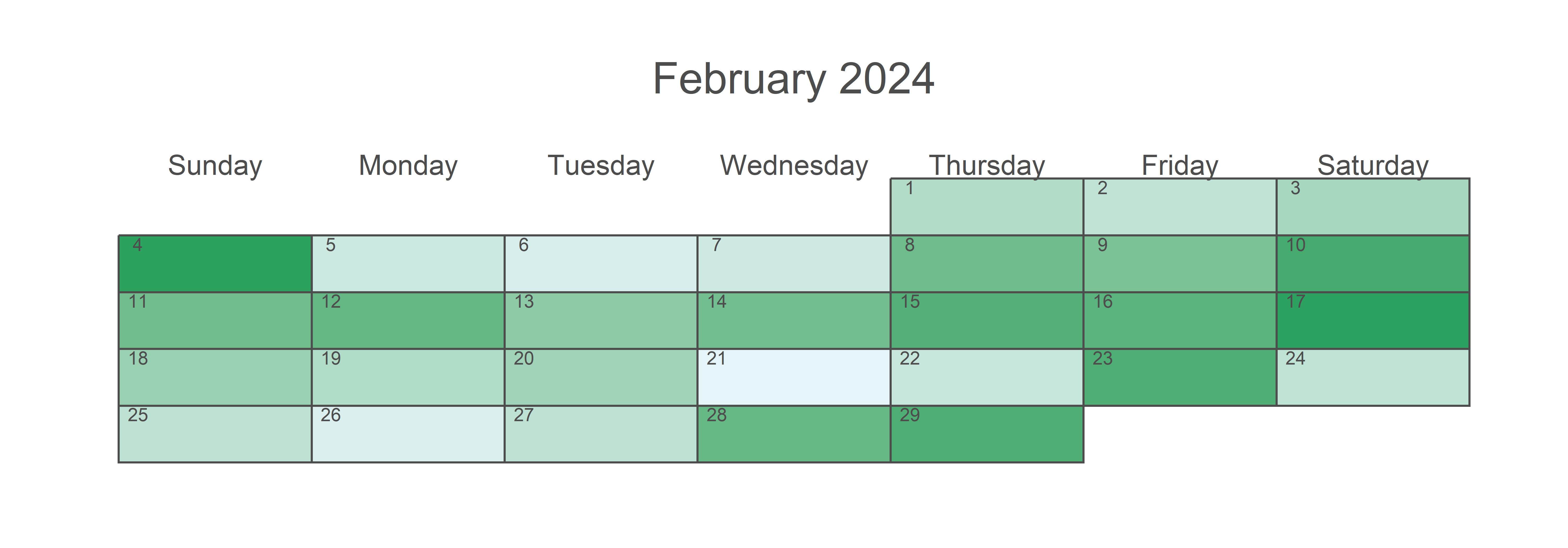

calendR(year = 2024, month = 3, 
        special.days = runif(31, 0, 100),
        gradient = TRUE,
        low.col = "#e5f5f9",
        special.col = "#2ca25f",
        title = "March 2024")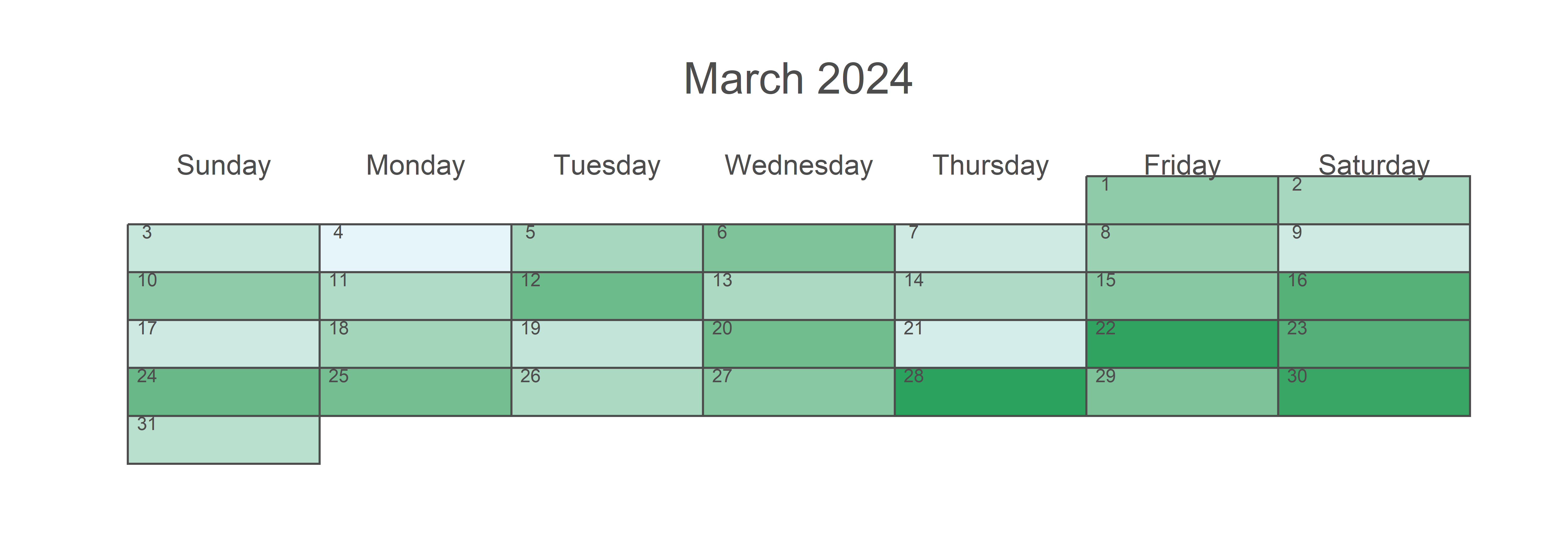

1.10 Gauge and Bullet Charts

Menampilkan pengukuran dalam format indikator atau skala.

# Buat Data Bullet Chart
bullet_data <- data.frame(
  Category = c("ALL", "Furniture", "Office Supplies", "Technology"),
  Target = c(1400000, 500000, 400000, 500000),
  Actual = c(900000, 350000, 300000, 400000),
  Range1 = c(500000, 200000, 150000, 250000),
  Range2 = c(1000000, 400000, 300000, 450000)
)

# Plot Bullet Chart
ggplot(bullet_data, aes(y = Category)) +
  geom_bar(aes(x = Target), stat = "identity", fill = "#D5E5A3", width = 0.6) +  
  geom_bar(aes(x = Range2), stat = "identity", fill = "#F4D03F", width = 0.6) +  
  geom_bar(aes(x = Range1), stat = "identity", fill = "#E74C3C", width = 0.6) +  
  geom_bar(aes(x = Actual), stat = "identity", fill = "black", width = 0.2) +  
  theme_minimal() +
  labs(title = "Bullet Chart: Target vs Actual", x = "Nilai (K)", y = "") +
  scale_x_continuous(labels = scales::comma)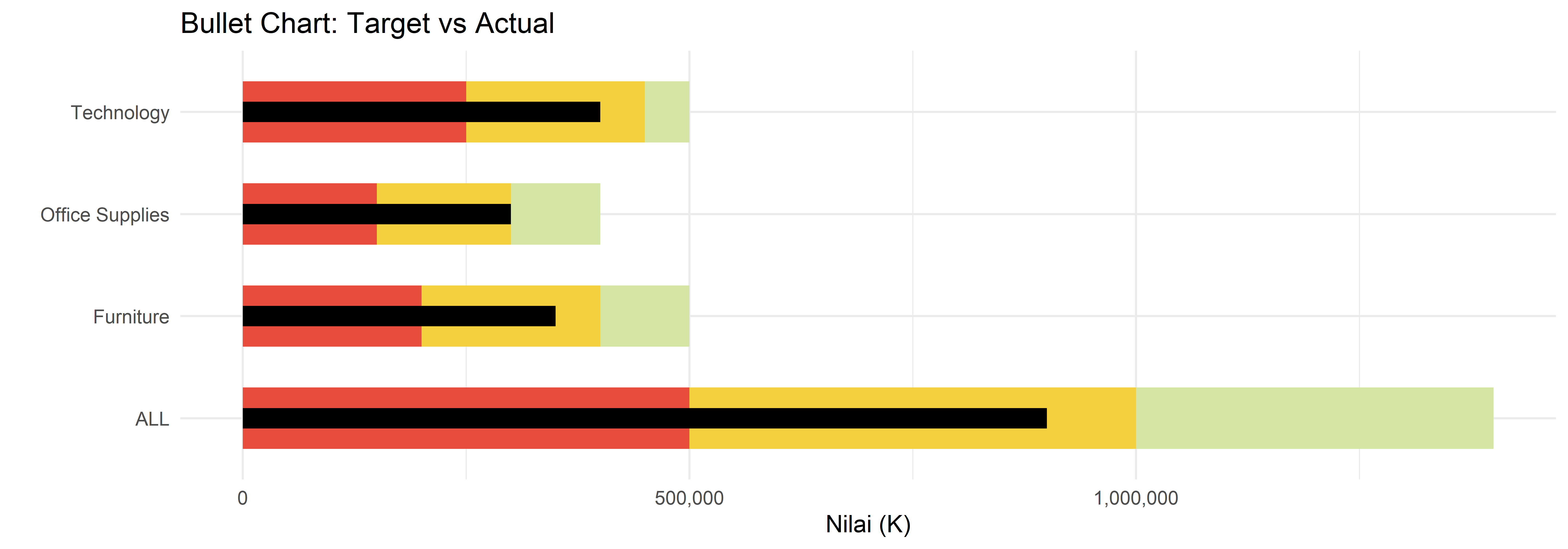

1.11 Bubble Comparison and Nested Bubbles

Digunakan untuk menunjukkan hierarki atau hubungan antar data.

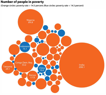
# Buat data contoh
bubble_data <- data.frame(
  Country = c("India", "Nigeria", "China", "Congo", "Indonesia", "Tanzania", "Kenya"),
  Population = c(208.1, 64.8, 100, 53.2, 15.1, 24.1, 17.8),
  PovertyRate = c(15, 16, 12, 18, 14, 17, 15)
)

# Warna berdasarkan tingkat kemiskinan
bubble_data$Color <- ifelse(bubble_data$PovertyRate >= 14.5, "orange", "blue")

# Plot Bubble Comparison
ggplot(bubble_data, aes(x = Population, y = PovertyRate, size = Population, fill = Color)) +
  geom_point(shape = 21, alpha = 0.7, color = "black") +
  scale_size(range = c(5, 25)) +
  scale_fill_manual(values = c("orange" = "orange", "blue" = "blue")) +
  geom_text(aes(label = Country), vjust = 1, color = "black", size = 5) +
  theme_minimal() +
  labs(title = "Bubble Comparison: Number of People in Poverty",
       subtitle = "Orange: Poverty rate > 14.5%, Blue: Poverty rate < 14.5%",
       x = "Population (millions)",
       y = "Poverty Rate (%)") +
  theme(legend.position = "none")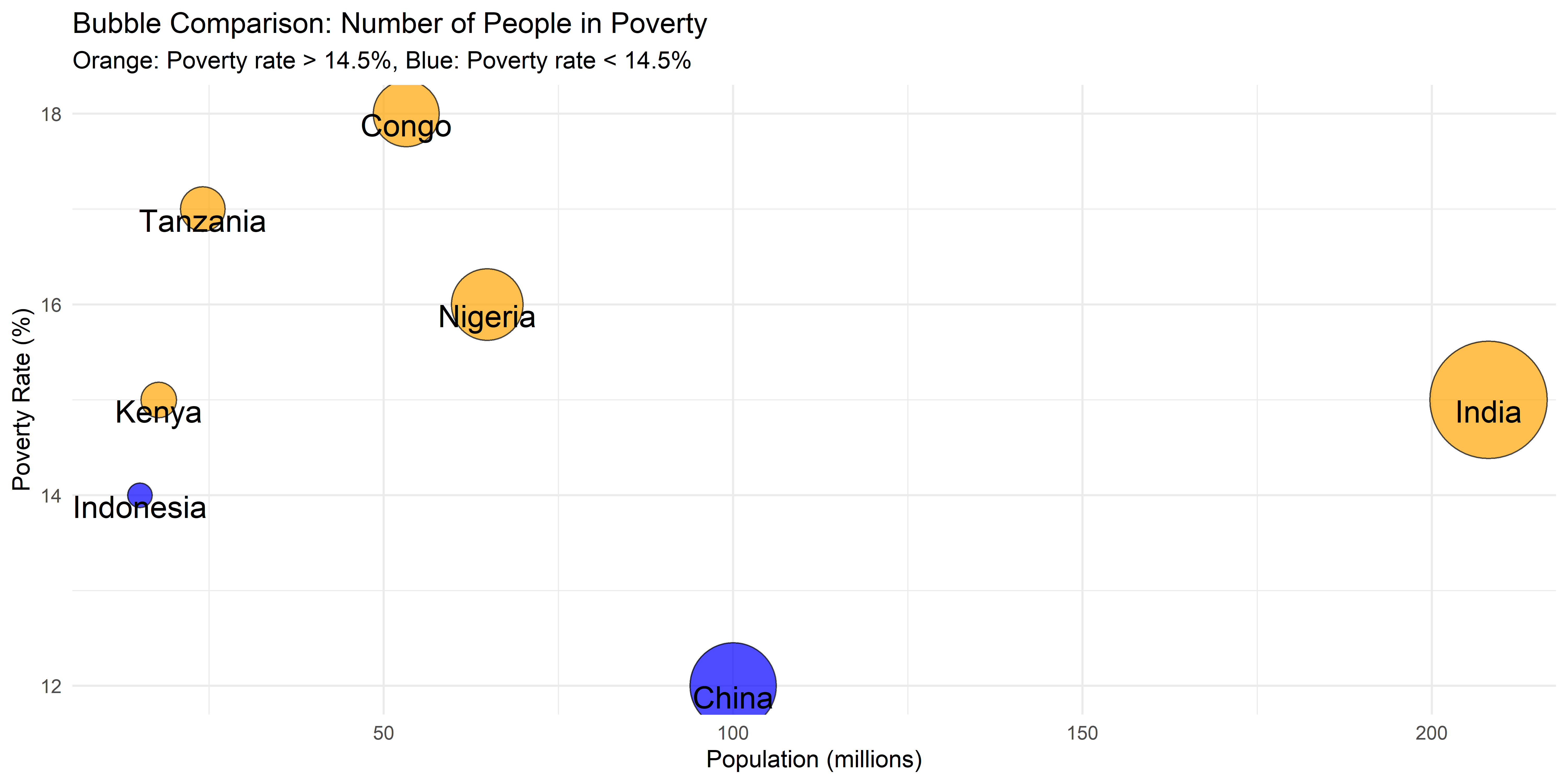

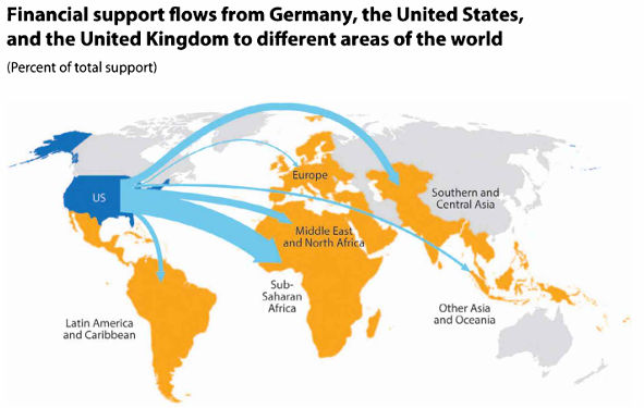
1.12 Sankey Diagram

Diagram aliran yang menunjukkan hubungan antar kategori.

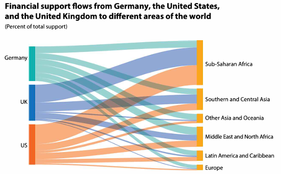
# Contoh data untuk aliran dukungan keuangan
sankey_data <- data.frame(
  Source = c("Germany", "Germany", "Germany", "Germany", "Germany", 
             "UK", "UK", "UK", "UK", "UK", 
             "US", "US", "US", "US", "US"),
  Target = c("Sub-Saharan Africa", "Southern and Central Asia", "Other Asia and Oceania", 
             "Middle East and North Africa", "Europe",
             "Sub-Saharan Africa", "Southern and Central Asia", "Other Asia and Oceania", 
             "Latin America and Caribbean", "Europe",
             "Sub-Saharan Africa", "Southern and Central Asia", "Middle East and North Africa", 
             "Latin America and Caribbean", "Europe"),
  Value = c(10, 15, 20, 30, 25, 12, 18, 14, 28, 28, 22, 16, 19, 23, 20)
)

# Plot Sankey Diagram menggunakan ggalluvial
ggplot(sankey_data, aes(axis1 = Source, axis2 = Target, y = Value)) +
  geom_alluvium(aes(fill = Source), width = 1/12) +
  geom_stratum(width = 1/12, fill = "gray") +
  geom_text(stat = "stratum", aes(label = after_stat(stratum)), size = 5) +
  theme_minimal() +
  labs(title = "Aliran Dukungan Keuangan",
       subtitle = "Dari Jerman, Inggris, dan AS ke Berbagai Wilayah Dunia",
       x = NULL, y = "Persentase Dukungan") +
  theme(legend.position = "none")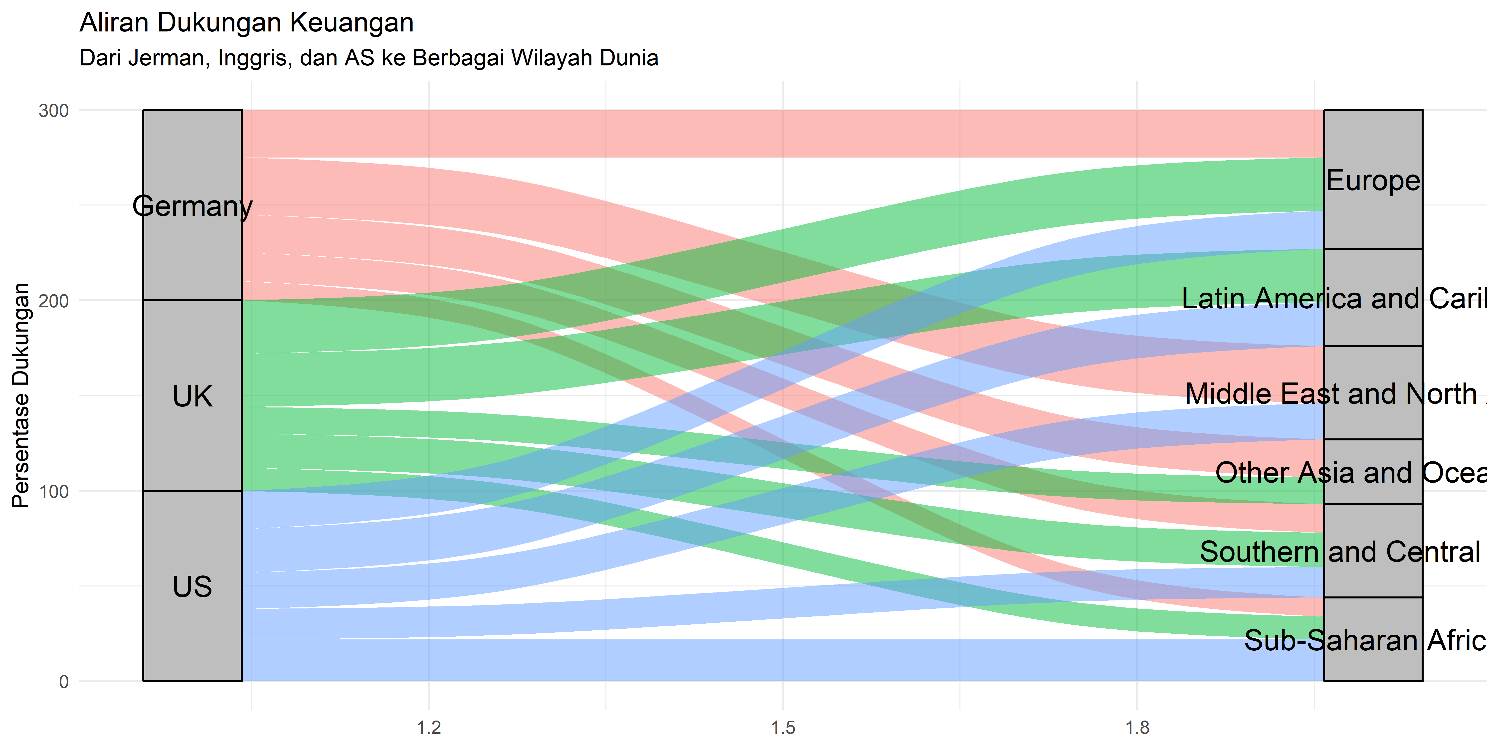

1.13 Waterfall Chart

Menunjukkan perubahan nilai dalam urutan kumulatif.