# Visualisasi Kualitatif
```{r setup, include=FALSE}
# Set Working Directory
opts_knit$set(root.dir = normalizePath("./"))
```
# **Qualitative** {#qualitative}
Visualisasi data kualitatif membantu menyampaikan informasi yang lebih deskriptif.
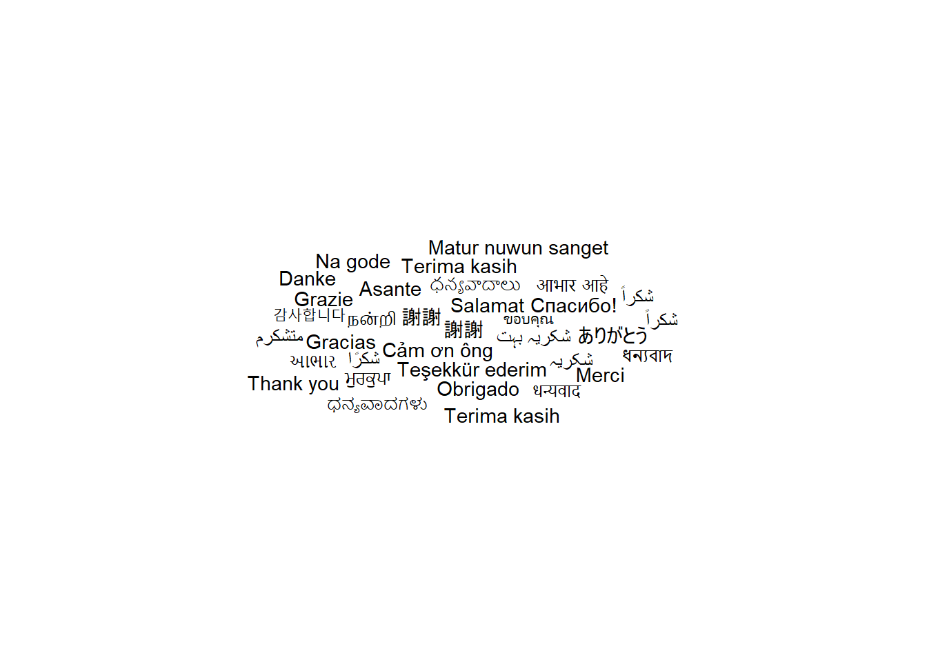
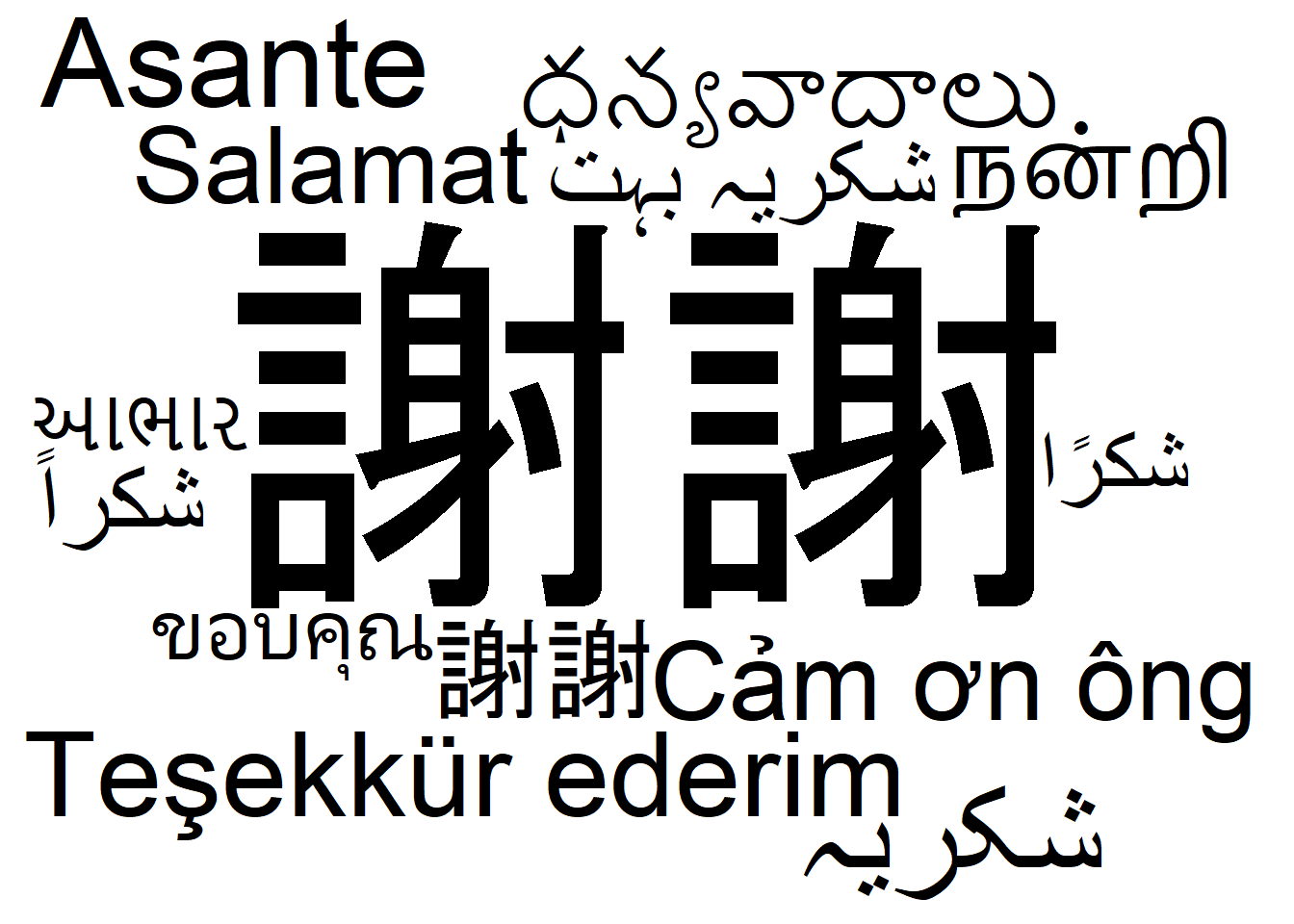
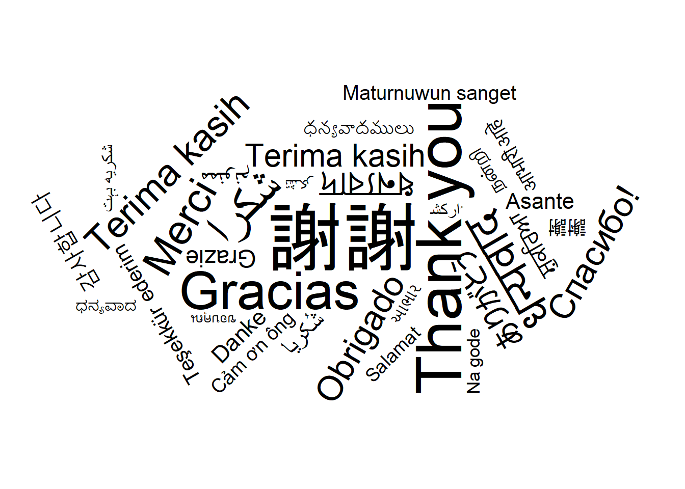
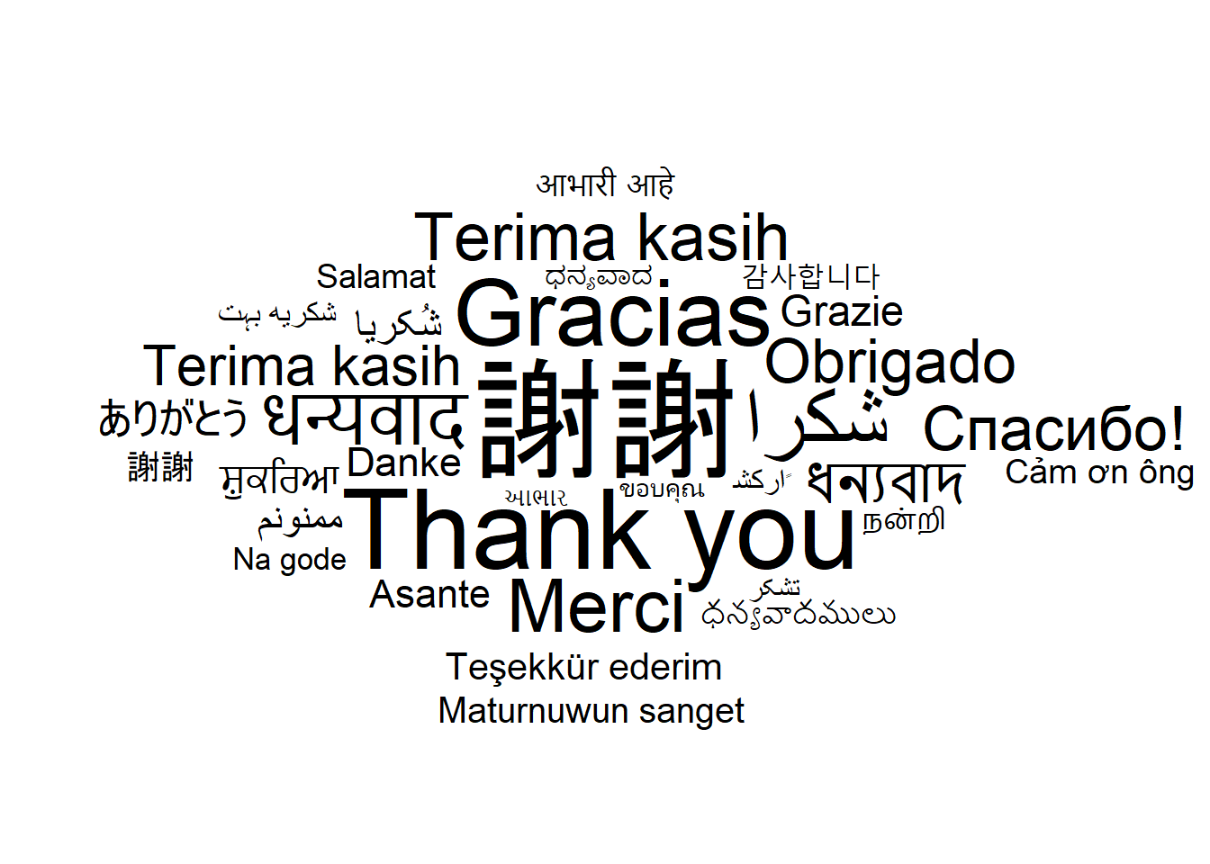
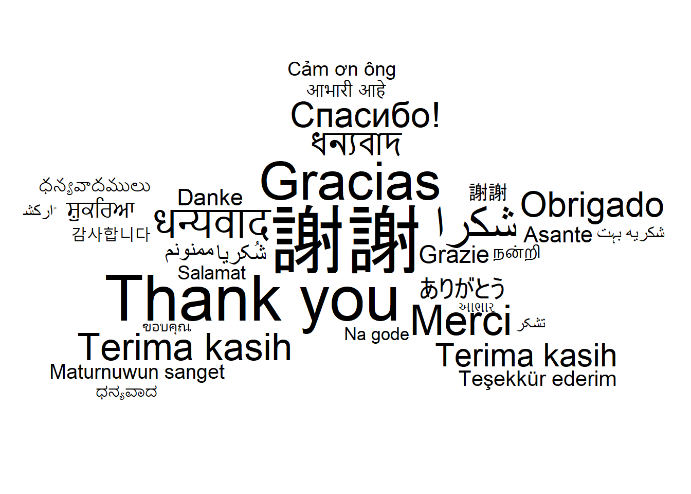
## Word Clouds and Specific Words {#word-clouds}
{width="198"}
Menampilkan distribusi kata dalam teks berdasarkan frekuensi penggunaannya.
```{r, message=FALSE}
df <- tibble(
  iso_639_3 = c("zho", "wuu", "vie", "urd", "tur", "tha",
                "tgl", "tel", "tam", "swa", "spa", "rus",
                "pus", "por", "pnb", "pan", "msa", "mar",
                "kor", "kan", "jpn", "jav", "ita", "ind",
                "hin", "hau", "guj", "fra", "fas", "eng",
                "deu", "ben", "arz", "ara"),
  word = c("謝謝", "謝謝", "Cảm ơn ông", "بہت شکریہ", "Teşekkür ederim", "ขอบคุณ",
           "Salamat", "ధన్యవాదాలు", "நன்றி", "Asante", "Gracias", "Спасибо!",
           "شكرًا", "Obrigado", "شکریہ", "ਮੁਰਕੁਪਾ", "Terima kasih", "आभार आहे",
           "감사합니다", "ಧನ್ಯವಾದಗಳು", "ありがとう", "Matur nuwun sanget", "Grazie", "Terima kasih",
           "धन्यवाद", "Na gode", "આભાર", "Merci", "متشكرم", "Thank you",
           "Danke", "ধন্যবাদ", "شكراً", "شكراً"),
  name = c("Chinese", "Wu Chinese", "Vietnamese", "Urdu", "Turkish", "Thai",
           "Tagalog", "Telugu", "Tamil", "Swahili", "Spanish", "Russian",
           "Pushto", "Portuguese", "Western Panjabi", "Panjabi", "Malay", "Marathi",
           "Korean", "Kannada", "Japanese", "Javanese", "Italian", "Indonesian",
           "Hindi", "Hausa", "Gujarati", "French", "Persian", "English",
           "German", "Bengali", "Egyptian Arabic", "Arabic"),
  native_speakers = c(1200, 80, 75, 67, 78.5, 28,
                      28, 81, 69, 8, 480, 154,
                      55, 220, 120, 120, 77, 83,
                      77.2, 69, 125, 82, 90, 43,
                      322, 43.7, 55, 76.8, 60, 400,
                      95, 260, 65, 245),
  speakers = c(1200, 80, 75, 67, 88, 72,
               73, 81, 77, 98, 555, 239,
               55, 243, 120, 120, 277, 83,
               77.2, 69, 125, 82, 114, 199,
               442, 63.2, 55, 350.8, 110, 800,
               107.5, 280, 65, 515)
)
```
```{r}
set.seed(1)
ggplot(df, aes(label = word)) +
  geom_text_wordcloud() +
  theme_minimal()
```
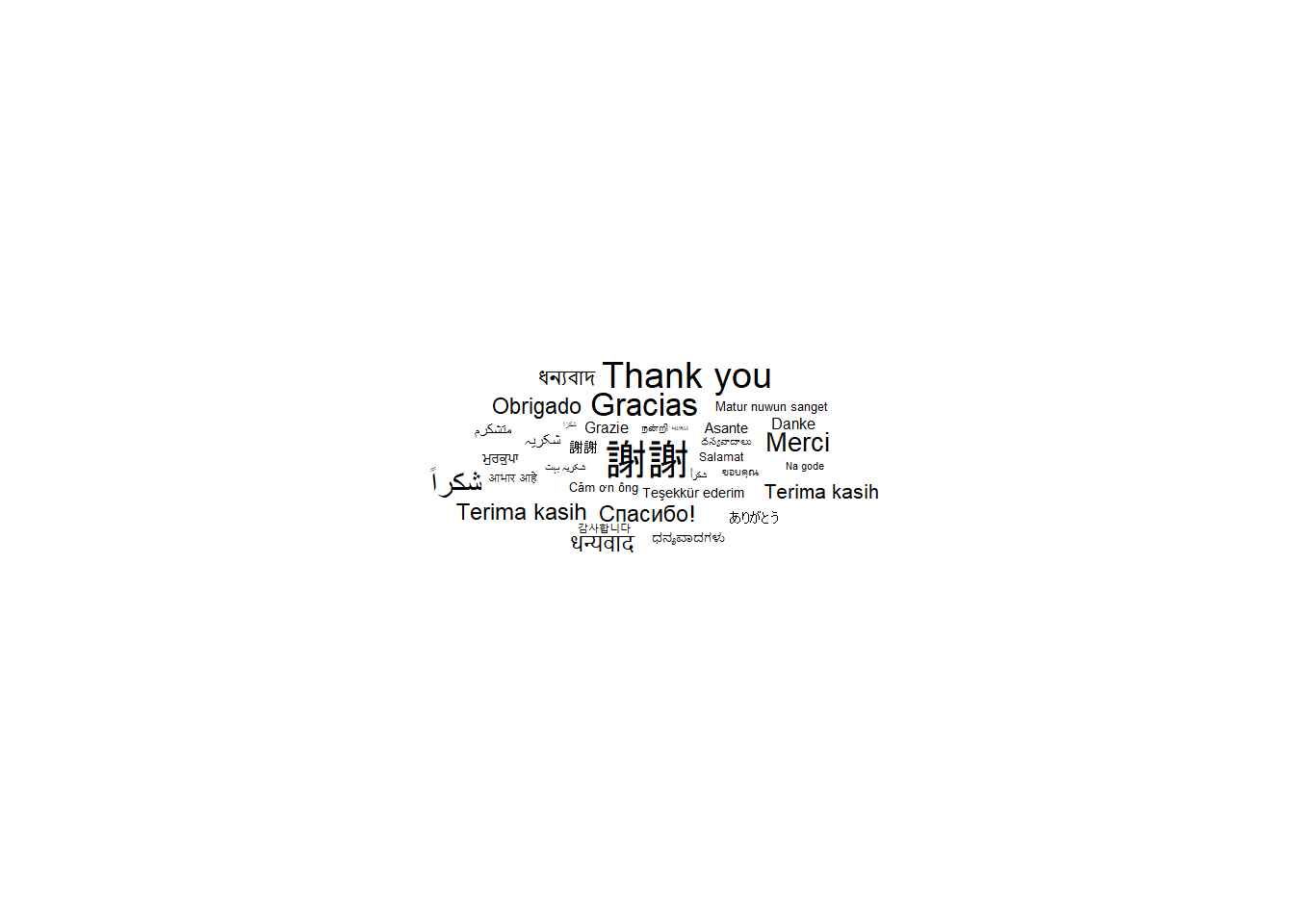
```{r}
set.seed(1)
ggplot(df, aes(label = word, size = speakers)) +
  geom_text_wordcloud() +
  theme_minimal()
```
```{r}
set.seed(1)
ggwordcloud(words = df$word, freq = df$speakers)
```
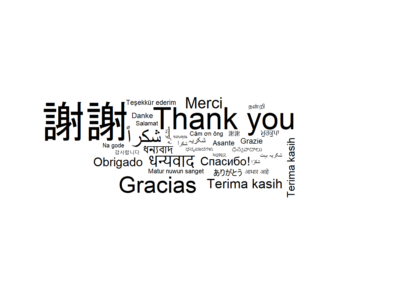
```{r}
set.seed(1)
ggplot(df, aes(label = word, size = speakers)) +
  geom_text_wordcloud() +
  scale_size_area(max_size = 20) +
  theme_minimal()
```
```{r}
set.seed(1)
ggplot(df, aes(label = word, size = speakers)) +
  geom_text_wordcloud(rm_outside = TRUE) +
  scale_size_area(max_size = 60) +
  theme_minimal()
```
```{r}
set.seed(1)

# Data
df <- thankyou_words_small
df$angle <- sample(c(0, 45, 60, 90, 120, 180), nrow(df), replace = TRUE)

ggplot(df, aes(label = word, size = speakers, angle = angle)) +
  geom_text_wordcloud() +
  scale_size_area(max_size = 20) +
  theme_minimal()
```
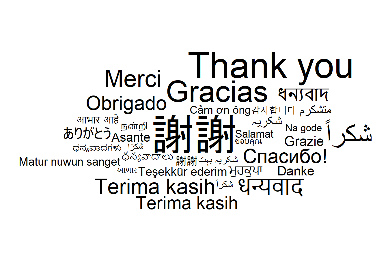
```{r}
set.seed(1)
ggplot(df, aes(label = word, size = speakers)) +
  geom_text_wordcloud(shape = "diamond") +
  scale_size_area(max_size = 20) +
  theme_minimal()
```
```{r}
set.seed(1)
ggplot(df, aes(label = word, size = speakers)) +
  geom_text_wordcloud(shape = "star") +
  scale_size_area(max_size = 20) +
  theme_minimal()
```
## Word Trees {#word-trees}
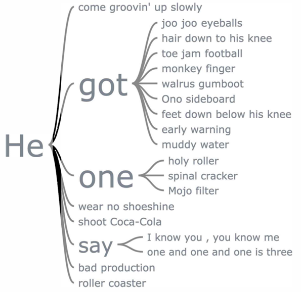{width="201"}
Menampilkan struktur hierarki dari kata atau frasa dalam teks.